1、线检测
水平:
| -1 | -1 | -1 |
| 2 | 2 | 2 |
| -1 | -1 | -1 |
+45°:
| 2 | -1 | -1 |
| -1 | 2 | -1 |
| -1 | -1 | 2 |
垂直:
| -1 | 2 | -1 |
| -1 | 2 | -1 |
| -1 | 2 | -1 |
当上面的模板在图像上移动时,就会对线(一个像素宽)的响应更加强烈。对于恒定的背景,使用第一个模板时,当水平线通过模板的中间一行可能产生更大的响应。响应,即指模板与图像进行卷积操作时,所得的乘积结果。
每个模板系数为0,表面在恒定亮度区域,模板响应为0.
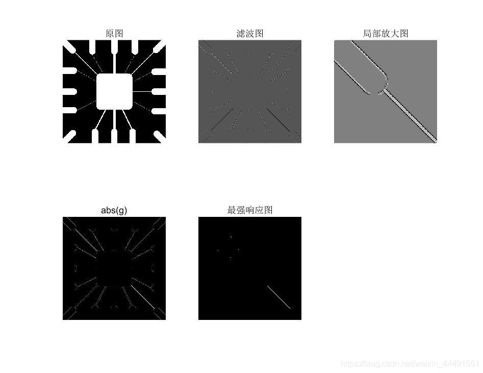
例:检测指定方向的线,比如是+45°。
使用第二个模板
%main

f=imread('E:\桌面\数字图像matlab\DIP3E_CH10_Original_Images\DIP3E_Original_Images_CH10\Fig1005(a)(wirebond_mask).tif');

w=[2 -1 -1;-1 2 -1;-1 -1 2];
g=imfilter(tofloat(f),w);%imfilter会给出与输入图像类型相同的输出,所以负值会被截掉,所以在这先将图像矩阵转换为浮点型。tofloat是书上给的,本质im2single函数,其实利用mat2gray也能得到一样的效果
imshow(g,[])
gtop=g(1:120,1:120);
gtop=pixeldup(gtop,4);
figure,imshow(gtop,[])
g=abs(g);
figure,imshow(g,[])
T=max(g(:));
g=g>=T;
figure,imshow(g);


%tofloat函数

function [out, revertclass]=tofloat(in)
%tofloat convert image to floating point

identity=@(x) x;
tosingle=@im2single;

table={'uint8', tosingle, @im2uint8
    'uint16', tosingle, @im2uint16
    'int16', tosingle, @im2int16
    'logical', tosingle, @logical
    'double', identity, identity
    'single', identity, identity};
classIndex=find(strcmp(class(in),table(:,1)));
if isempty(classIndex)
error('Unsupported inut image class.')
end

out=table{classIndex,2}(in);
revertclass=table{classIndex,3};

%pixeldup函数

function B=pixeldup(A,m,n)%pixeldup用来重复像素的,在水平方向复制m倍,在垂直方向复制n倍,m,n必须为整数,n没有赋值默认为m
%检查输入参数个数
if nargin<2
    error('At least two inputs are required.');
end
if nargin==2
    n=m;
end
u=1:size(A,1);%产生一个向量,其向量中元素的个数为A的行数
%复制向量中每个元素m次
m=round(m);%防止m为非整数
u=u(ones(1,m),:);
u=u(:);
%在垂直方向重复操作
v=1:size(A,2);
n=round(n);
v=v(ones(1,n),:);
v=v(:);
B=A(u,v);
结果如下:
2、使用edge函数
目前为止,最通用的边缘检测是 检测亮度的不连续性。利用一阶或者二阶导数检测。
sobel的一般语法形式:[g,t]=edge(f,'sobel',T,dir)
f是输入图像,T是阈值,dir是边缘检测首选方向,‘horizontal’,‘vertical’,‘both’(默认),如果T指定了值,则t=T,如果没有,就自动计算得到阈值,并让t等于这个值。
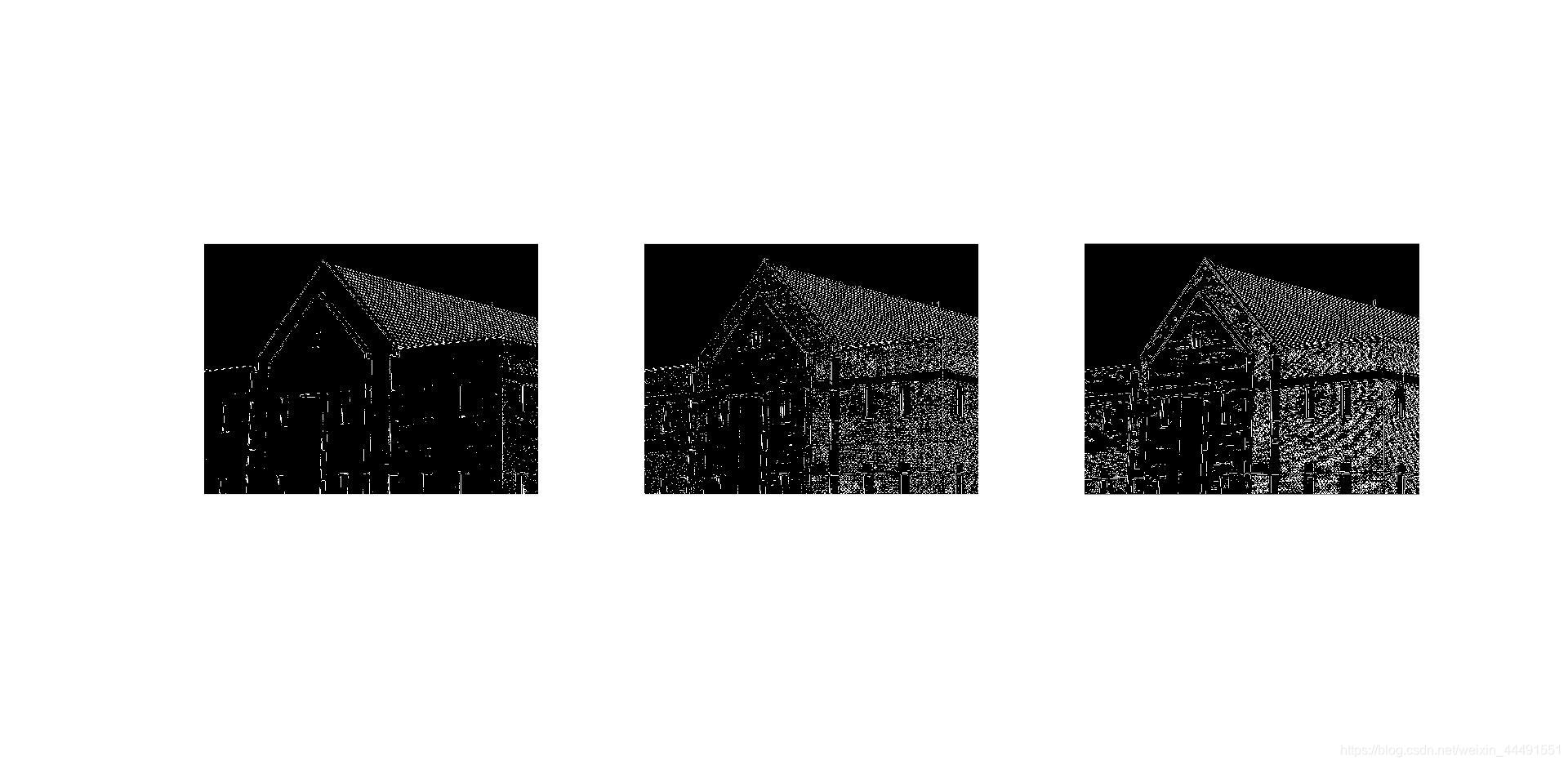
例:Sobel边缘检测算子
clc
clear

f=imread('E:\桌面\数字图像matlab\DIP3E_CH10_Original_Images\DIP3E_Original_Images_CH10\Fig1016(a)(building_original).tif');
subplot(231),imshow(f),title('原图')

%阈值自动计算,首选方向选择垂直
[gv,t]=edge(f,'sobel','vertical');
subplot(232),imshow(gv),title('sobel v')

%阈值0.15,首选方向选择垂直
gv2=edge(f,'sobel',0.15,'vertical');
subplot(233),imshow(gv2),title('sobel T=0.15 v')

%阈值0.15,首选方向默认both
gboth=edge(f,'sobel',0.15);
subplot(234),imshow(gboth),title('sobel T=0.15 both')

%-45
wneg45=[-2 -1 0;-1 0 1;0 1 2];
gneg45=imfilter(tofloat(f),wneg45,'replicate');
T=0.3*max(abs(gneg45(:)));
gneg45=gneg45>=T;
subplot(235),imshow(gneg45),title('-45')

%+45
wpos45=[0 1 2;-1 0 1;-2 -1 0];
gpos45=imfilter(tofloat(f),wpos45,'replicate');
T=0.3*max(abs(gpos45(:)));
gpos45=gpos45>=T;
subplot(236),imshow(gpos45),title('+45')
结果如下:

sobel、LoG、Canny边缘检测算子的比较
首先都采取默认参数,得到结果,然后再自行设定阈值等参数:
f=imread('E:\桌面\数字图像matlab\DIP3E_CH10_Original_Images\DIP3E_Original_Images_CH10\Fig1016(a)(building_original).tif');
f=tofloat(f);
[sobel_def,ts]=edge(f,'sobel');
[Log_def,tlog]=edge(f,'log');
[Canny_def,tc]=edge(f,'canny');

subplot(131),imshow(sobel_def);
subplot(132),imshow(Log_def);
subplot(133),imshow(Canny_def);

sobel_best=edge(f,'sobel',0.05);
Log_best=edge(f,'log',0.003,2.25);
Canny_best=edge(f,'canny',[0.04 0.1],1.5);
figure
subplot(131),imshow(sobel_best);
subplot(132),imshow(Log_best);
subplot(133),imshow(Canny_best);
默认参数:
自设参数:
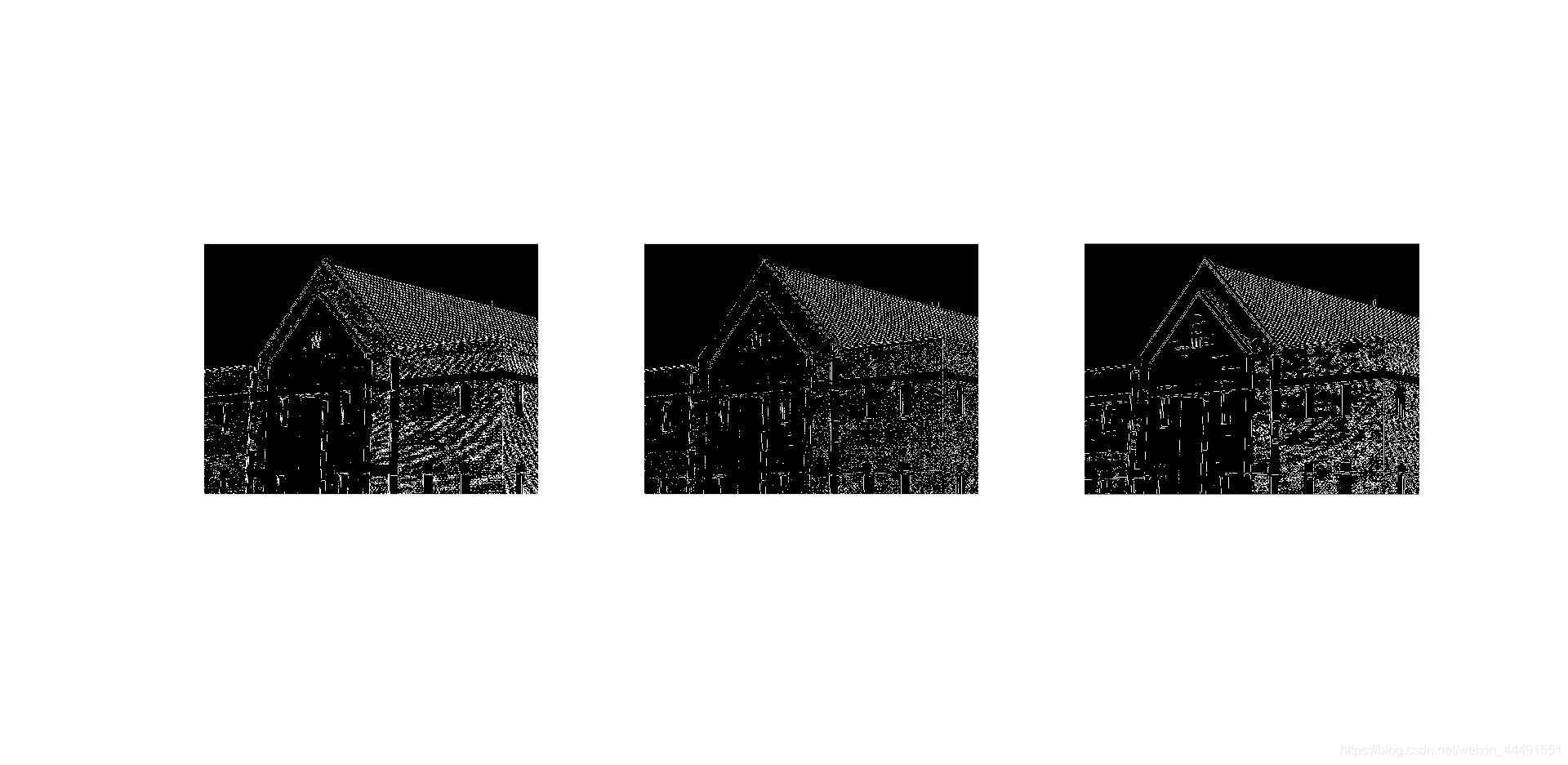
有时候需要自行不断调整参数,才能得到更好的结果。
3、使用霍夫变换的边缘检测
用前面Canny检测算子得到的二值图像,下图所示,进行霍夫变换和连接线。
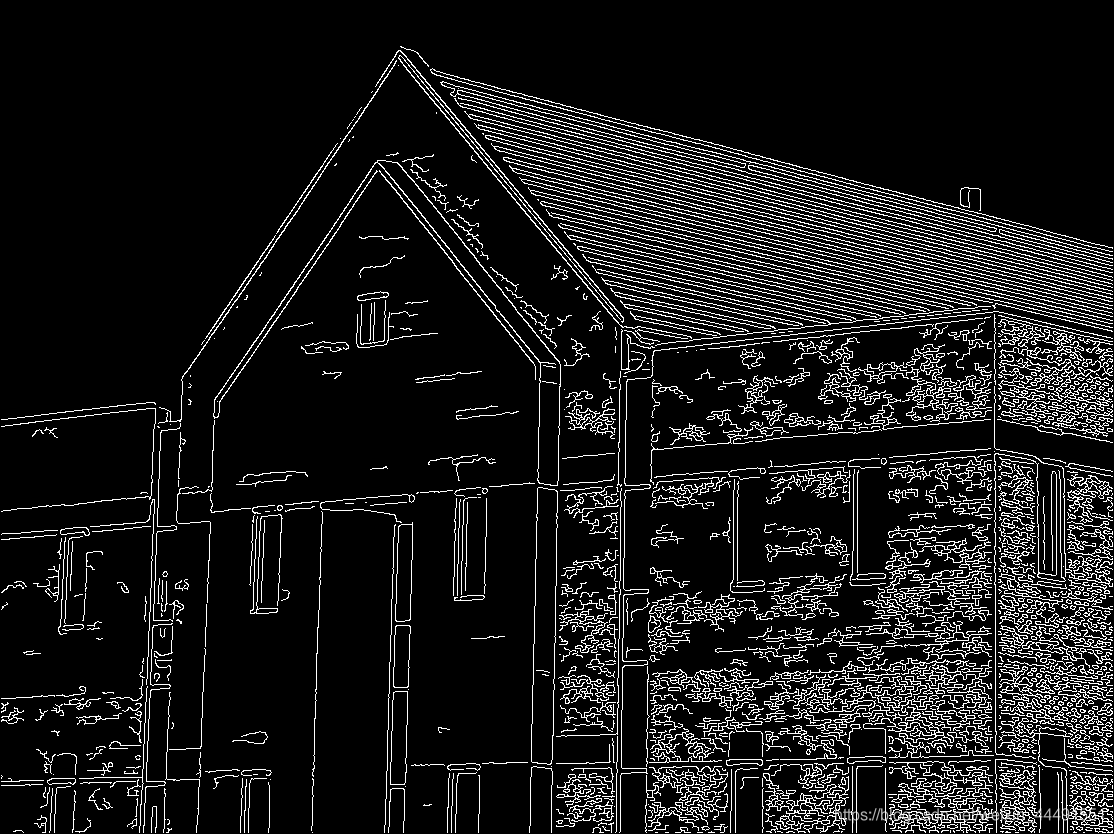
f=imread('E:\桌面\Canny.bmp');
[H,theta,rho]=hough(f,'ThetaResolution',0.2);
imshow(H,[],'XData',theta,'YData',rho,'InitialMagnification','fit');
axis on,axis normal
xlabel('\theta'),ylabel('\rho')

peaks=houghpeaks(H,5);
hold on
plot(theta(peaks(:,2)),rho(peaks(:,1)),...
    'linestyle','none','marker','s','color','w')
lines=houghlines(f,theta,rho,peaks);
figure,imshow(f),hold on
for k=1:length(lines)
    xy=[lines(k).point1;lines(k).point2];
    plot(xy(:,1),xy(:,2),'Linewidth',4,'Color',[.8 .8 .8]);
end
结果如下:
下图中有5个方块,说明找到了5个峰值点,也就是二维累加数组最大值点,也就是参数空间中所过该点的曲线数目最多,对应到坐标空间中,就是共线点最多,就可以视为边缘。
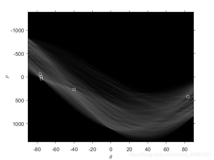
霍夫变换需要二值输入,所以需要先进行一步边缘检测,如canny检测。
更多的介绍可看这篇文章经典霍夫变换。
版权声明:本文为weixin_44491551原创文章,遵循CC 4.0 BY-SA版权协议,转载请附上原文出处链接和本声明。