一、SIFT算法原理和步骤
1.1 SIFT特征提取原理
Sfit算法的实质是在不同的尺度空间上查找关键点(特征点),计算关键点的大小、方向、尺度信息,利用这些信息组成关键点对特征点进行描述的问题。Sift所查找的关键点都是一些十分突出,不会因光照,仿射便函和噪声等因素而变换的“稳定”特征点,如角点、边缘点、暗区的亮点以及亮区的暗点等。
1.2 SIFT特征匹配原理
匹配的过程就是对比这些特征点的过程,这个流程可以用下图表述:
1.3 SIFT特征提取和匹配具体步骤
- 生成高斯差分金字塔(DOG金字塔),尺度空间构建
- 空间极值点检测(关键点的初步查探)
- 稳定关键点的精确定位
- 稳定关键点方向信息分配
- 关键点描述
- 特征点匹配
二、实验
2.1 SIFT特征提取
2.1.1 SIFT特征提取实现代码
# -*- coding: utf-8 -*-
from PIL import Image
from pylab import *
from PCV.localdescriptors import sift
from PCV.localdescriptors import harris

# 添加中文字体支持
from matplotlib.font_manager import FontProperties
font = FontProperties(fname=r"c:\windows\fonts\SimSun.ttc", size=14)

imname = 'C:\image\sift6.png'
im = array(Image.open(imname).convert('L'))
sift.process_image(imname, 'empire.sift')
l1, d1 = sift.read_features_from_file('empire.sift')

figure()
gray()
subplot(131)
sift.plot_features(im, l1, circle=False)
title(u'SIFT特征',fontproperties=font)
subplot(132)
sift.plot_features(im, l1, circle=True)
title(u'用圆圈表示SIFT特征尺度',fontproperties=font)

# 检测harris角点
harrisim = harris.compute_harris_response(im)

subplot(133)
filtered_coords = harris.get_harris_points(harrisim, 6, 0.1)
imshow(im)
plot([p[1] for p in filtered_coords], [p[0] for p in filtered_coords], '*')
axis('off')
title(u'Harris角点',fontproperties=font)

show()
sift.plot_features(im, l1, circle=False):寻找图像中的Sift特征
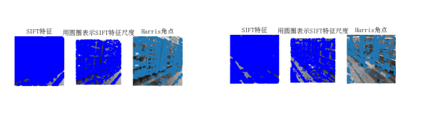
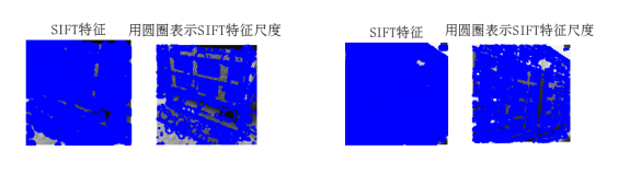
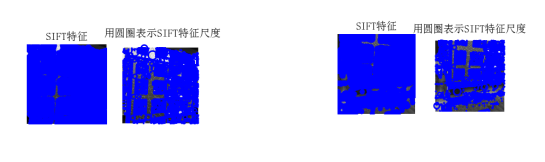
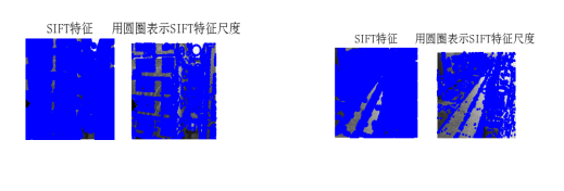
2.1.2 SIFT特征提取实现结果
数据集准备:准备了十五张来自不同场景的图片构成一个小数据集


1-6张图片的特征提取

7-15张图片特征提取
2.2 SIFT特征匹配
2.2.1 SIFT特征匹配实现代码
from PIL import Image
from pylab import *
import sys
from PCV.localdescriptors import sift


if len(sys.argv) >= 3:
  im1f, im2f = sys.argv[1], sys.argv[2]
else:
#  im1f = '../data/sf_view1.jpg'
#  im2f = '../data/sf_view2.jpg'
  im1f = 'C:\image\sift1.png'
  im2f = 'C:\image\sift2.png'
#  im1f = '../data/climbing_1_small.jpg'
#  im2f = '../data/climbing_2_small.jpg'
im1 = array(Image.open(im1f))
im2 = array(Image.open(im2f))

sift.process_image(im1f, 'out_sift_1.txt')
l1, d1 = sift.read_features_from_file('out_sift_1.txt')
figure()
gray()
subplot(121)
sift.plot_features(im1, l1, circle=False)

sift.process_image(im2f, 'out_sift_2.txt')
l2, d2 = sift.read_features_from_file('out_sift_2.txt')
subplot(122)
sift.plot_features(im2, l2, circle=False)

#matches = sift.match(d1, d2)
matches = sift.match_twosided(d1, d2)
print ('{} matches'.format(len(matches.nonzero()[0])))

figure()
gray()
sift.plot_matches(im1, im2, l1, l2, matches, show_below=True)
show()
matches = sift.match_twosided(d1, d2):对两幅图中的SIFT特征进行匹配:
2.2.2 SIFT特征匹配实现结果

给定两张角度不同的场景照片,进行sift描述子匹配。特征点的匹配是通过计算两组特征点的128维的关键点的欧式距离实现的。欧式距离越小,则相似度越高,当欧式距离小于设定的阈值时,可以判定为匹配成功。
2.3 SIFT特征检索
2.3.1 SIFT特征检索实现代码
# -*- coding: utf-8 -*-
from PIL import Image
from pylab import *
from numpy import *
import os
from PCV.tools.imtools import get_imlist  # 导入原书的PCV模块
import matplotlib.pyplot as plt  # plt 用于显示图片
import matplotlib.image as mpimg  # mpimg 用于读取图片


def process_image(imagename, resultname, params="--edge-thresh 10 --peak-thresh 5"):
    """ 处理一幅图像,然后将结果保存在文件中"""
    if imagename[-3:] != 'pgm':
        # 创建一个pgm文件
        im = Image.open(imagename).convert('L')
        im.save('tmp.pgm')
        imagename = 'tmp.pgm'
    cmmd = str("sift " + imagename + " --output=" + resultname + " " + params)
    os.system(cmmd)
    print ('processed', imagename, 'to', resultname)


def read_features_from_file(filename):
    """读取特征属性值,然后将其以矩阵的形式返回"""
    f = loadtxt(filename)
    return f[:, :4], f[:, 4:]  # 特征位置,描述子


def write_featrues_to_file(filename, locs, desc):
    """将特征位置和描述子保存到文件中"""
    savetxt(filename, hstack((locs, desc)))


def plot_features(im, locs, circle=False):
    """显示带有特征的图像
       输入:im(数组图像),locs(每个特征的行、列、尺度和朝向)"""

    def draw_circle(c, r):
        t = arange(0, 1.01, .01) * 2 * pi
        x = r * cos(t) + c[0]
        y = r * sin(t) + c[1]
        plot(x, y, 'b', linewidth=2)

    imshow(im)
    if circle:
        for p in locs:
            draw_circle(p[:2], p[2])
    else:
        plot(locs[:, 0], locs[:, 1], 'ob')
    axis('off')


def match(desc1, desc2):
    """对于第一幅图像中的每个描述子,选取其在第二幅图像中的匹配
    输入:desc1(第一幅图像中的描述子),desc2(第二幅图像中的描述子)"""
    desc1 = array([d / linalg.norm(d) for d in desc1])
    desc2 = array([d / linalg.norm(d) for d in desc2])
    dist_ratio = 0.6
    desc1_size = desc1.shape
    matchscores = zeros((desc1_size[0], 1), 'int')
    desc2t = desc2.T  # 预先计算矩阵转置
    for i in range(desc1_size[0]):
        dotprods = dot(desc1[i, :], desc2t)  # 向量点乘
        dotprods = 0.9999 * dotprods
        # 反余弦和反排序,返回第二幅图像中特征的索引
        indx = argsort(arccos(dotprods))
        # 检查最近邻的角度是否小于dist_ratio乘以第二近邻的角度
        if arccos(dotprods)[indx[0]] < dist_ratio * arccos(dotprods)[indx[1]]:
            matchscores[i] = int(indx[0])
    return matchscores


def match_twosided(desc1, desc2):
    """双向对称版本的match()"""
    matches_12 = match(desc1, desc2)
    matches_21 = match(desc2, desc1)
    ndx_12 = matches_12.nonzero()[0]
    # 去除不对称的匹配
    for n in ndx_12:
        if matches_21[int(matches_12[n])] != n:
            matches_12[n] = 0
    return matches_12


def appendimages(im1, im2):
    """返回将两幅图像并排拼接成的一幅新图像"""
    # 选取具有最少行数的图像,然后填充足够的空行
    rows1 = im1.shape[0]
    rows2 = im2.shape[0]
    if rows1 < rows2:
        im1 = concatenate((im1, zeros((rows2 - rows1, im1.shape[1]))), axis=0)
    elif rows1 > rows2:
        im2 = concatenate((im2, zeros((rows1 - rows2, im2.shape[1]))), axis=0)
    return concatenate((im1, im2), axis=1)


def plot_matches(im1, im2, locs1, locs2, matchscores, show_below=True):
    """ 显示一幅带有连接匹配之间连线的图片
        输入:im1, im2(数组图像), locs1,locs2(特征位置),matchscores(match()的输出),
        show_below(如果图像应该显示在匹配的下方)
    """
    im3 = appendimages(im1, im2)
    if show_below:
        im3 = vstack((im3, im3))
    imshow(im3)
    cols1 = im1.shape[1]
    for i in range(len(matchscores)):
        if matchscores[i] > 0:
            plot([locs1[i, 0], locs2[matchscores[i, 0], 0] + cols1], [locs1[i, 1], locs2[matchscores[i, 0], 1]], 'c')
    axis('off')


# 获取project2_data文件夹下的图片文件名(包括后缀名)
filelist = get_imlist('C:/image/')

# 输入的图片
im1f = 'C:\image\sift1.png'
im1 = array(Image.open(im1f))
process_image(im1f, 'out_sift_1.txt')
l1, d1 = read_features_from_file('out_sift_1.txt')

i = 0
num = [0] * 30  # 存放匹配值
for infile in filelist:  # 对文件夹下的每张图片进行如下操作
    im2 = array(Image.open(infile))
    process_image(infile, 'out_sift_2.txt')
    l2, d2 = read_features_from_file('out_sift_2.txt')
    matches = match_twosided(d1, d2)
    num[i] = len(matches.nonzero()[0])
    i = i + 1
    print ('{} matches'.format(num[i - 1]))  # 输出匹配值

i = 1
figure()
while i < 4:  # 循环三次,输出匹配最多的三张图片
    index = num.index(max(num))
    print (index, filelist[index])
    lena = mpimg.imread(filelist[index])  # 读取当前匹配最大值的图片
    # 此时 lena 就已经是一个 np.array 了,可以对它进行任意处理
    # lena.shape  # (512, 512, 3)
    subplot(1, 3, i)
    plt.imshow(lena)  # 显示图片
    plt.axis('off')  # 不显示坐标轴
    num[index] = 0  # 将当前最大值清零
    i = i + 1
show()
2.3.2 SIFT特征检索实现结果
- 输出:匹配度较高的前三张图片

2.4 地理标记图像匹配
2.4.1 地理标记图像匹配实现代码
在进行实验前要先安装完GraphViz,否则会出现下图错误
在该行代码imlist = imtools.get_imlist(download_path) 出现错误,导致程序运行结果为空
通过print(imlist)输出可知列表中并没有图片名称。
在将图片后缀的大写修改为小写后,成功输出结果。
# -*- coding: utf-8 -*-
from pylab import *
from PIL import Image
from PCV.localdescriptors import sift
from PCV.tools import imtools
import pydot

import os

os.environ['PATH'] = os.environ['PATH'] + (';c:\\Program Files (x86)\\Graphviz2.38\\bin\\')


""" This is the example graph illustration of matching images from Figure 2-10.
To download the images, see ch2_download_panoramio.py."""

#download_path = "panoimages"  # set this to the path where you downloaded the panoramio images
#path = "/FULLPATH/panoimages/"  # path to save thumbnails (pydot needs the full system path)

download_path = "C:/image"  # set this to the path where you downloaded the panoramio images
path = "C:/image/"  # path to save thumbnails (pydot needs the full system path)

# list of downloaded filenames
imlist = imtools.get_imlist(download_path)
nbr_images = len(imlist)

# extract features
featlist = [imname[:-3] + 'sift' for imname in imlist]
for i, imname in enumerate(imlist):
    sift.process_image(imname, featlist[i])

matchscores = zeros((nbr_images, nbr_images))

for i in range(nbr_images):
    for j in range(i, nbr_images):  # only compute upper triangle
        print ('comparing ', imlist[i], imlist[j])
        l1, d1 = sift.read_features_from_file(featlist[i])
        l2, d2 = sift.read_features_from_file(featlist[j])
        matches = sift.match_twosided(d1, d2)
        nbr_matches = sum(matches > 0)
        print ('number of matches = ', nbr_matches)
        matchscores[i, j] = nbr_matches
print ("The match scores is: \n", matchscores)

# copy values
for i in range(nbr_images):
    for j in range(i + 1, nbr_images):  # no need to copy diagonal
        matchscores[j, i] = matchscores[i, j]

#可视化

threshold = 2  # min number of matches needed to create link

g = pydot.Dot(graph_type='graph')  # don't want the default directed graph

for i in range(nbr_images):
    for j in range(i + 1, nbr_images):
        if matchscores[i, j] > threshold:
            # first image in pair
            im = Image.open(imlist[i])
            im.thumbnail((100, 100))
            filename = path + str(i) + '.png'
            im.save(filename)  # need temporary files of the right size
            g.add_node(pydot.Node(str(i), fontcolor='transparent', shape='rectangle', image=filename))

            # second image in pair
            im = Image.open(imlist[j])
            im.thumbnail((100, 100))
            filename = path + str(j) + '.png'
            im.save(filename)  # need temporary files of the right size
            g.add_node(pydot.Node(str(j), fontcolor='transparent', shape='rectangle', image=filename))

            g.add_edge(pydot.Edge(str(i), str(j)))
g.write_png('whitehouse.png')
2.4.2 地理标记图像匹配实现结果

2.4.3地理标记图像匹配实验小结
通过上述实验结果对比可以发现,不同视点的图像仍然可以正确匹配出来。所以通过利用局部描述子(即SIFT描述子)对地理标记图像进行匹配,可以解决不同角度(不同视点)拍摄的图像匹配问题。但该算法也存在不足,在于当遮挡物较多时,仅能匹配到图像中的标志性建筑例如建筑大楼此类,最终匹配结果十分狭窄。并因为此次实验拍摄的图像特征点周围纹理相近,颜色相近,造成分类效果不佳。可以推测当拍摄图片特征点周围纹理多且复杂,如草地等,分类效果也不佳。
三、经过RANSAC的SIFT匹配
3.1 RANSAC原理
OpenCV中滤除误匹配对采用RANSAC算法寻找一个最佳单应性矩阵H,矩阵大小为3×3。RANSAC目的是找到最优的参数矩阵使得满足该矩阵的数据点个数最多,通常令h33=1来归一化矩阵。由于单应性矩阵有8个未知参数,至少需要8个线性方程求解,对应到点位置信息上,一组点对可以列出两个方程,则至少包含4组匹配点对。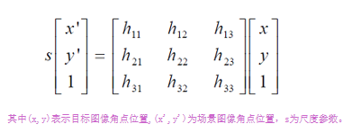
3.2 RANSAC算法步骤
RANSAC算法步骤:
1. 随机从数据集中随机抽出4个样本数据 (此4个样本之间不能共线),计算出变换矩阵H,记为模型M;
2. 计算数据集中所有数据与模型M的投影误差,若误差小于阈值,加入内点集 I
3. 如果当前内点集 I 元素个数大于最优内点集 I_best , 则更新 I_best = I,同时更新迭代次数k ;
4. 如果迭代次数大于k,则退出 ; 否则迭代次数加1,并重复上述步骤;
注:迭代次数k在不大于最大迭代次数的情况下,是在不断更新而不是固定的;
3.3 经过RANSAC的SIFT匹配实现代码
# -*- coding: utf-8 -*-
import cv2
import numpy as np
import random

def compute_fundamental(x1, x2):
    n = x1.shape[1]
    if x2.shape[1] != n:
        raise ValueError("Number of points don't match.")

    # build matrix for equations
    A = np.zeros((n, 9))
    for i in range(n):
        A[i] = [x1[0, i] * x2[0, i], x1[0, i] * x2[1, i], x1[0, i] * x2[2, i],
                x1[1, i] * x2[0, i], x1[1, i] * x2[1, i], x1[1, i] * x2[2, i],
                x1[2, i] * x2[0, i], x1[2, i] * x2[1, i], x1[2, i] * x2[2, i]]

    # compute linear least square solution
    U, S, V = np.linalg.svd(A)
    F = V[-1].reshape(3, 3)

    # constrain F
    # make rank 2 by zeroing out last singular value
    U, S, V = np.linalg.svd(F)
    S[2] = 0
    F = np.dot(U, np.dot(np.diag(S), V))

    return F / F[2, 2]


def compute_fundamental_normalized(x1, x2):
    """    Computes the fundamental matrix from corresponding points
        (x1,x2 3*n arrays) using the normalized 8 point algorithm. """

    n = x1.shape[1]
    if x2.shape[1] != n:
        raise ValueError("Number of points don't match.")

    # normalize image coordinates
    x1 = x1 / x1[2]
    mean_1 = np.mean(x1[:2], axis=1)
    S1 = np.sqrt(2) / np.std(x1[:2])
    T1 = np.array([[S1, 0, -S1 * mean_1[0]], [0, S1, -S1 * mean_1[1]], [0, 0, 1]])
    x1 = np.dot(T1, x1)

    x2 = x2 / x2[2]
    mean_2 = np.mean(x2[:2], axis=1)
    S2 = np.sqrt(2) / np.std(x2[:2])
    T2 = np.array([[S2, 0, -S2 * mean_2[0]], [0, S2, -S2 * mean_2[1]], [0, 0, 1]])
    x2 = np.dot(T2, x2)

    # compute F with the normalized coordinates
    F = compute_fundamental(x1, x2)
    # print (F)
    # reverse normalization
    F = np.dot(T1.T, np.dot(F, T2))

    return F / F[2, 2]

def randSeed(good, num = 8):
    '''
    :param good: 初始的匹配点对
    :param num: 选择随机选取的点对数量
    :return: 8个点对list
    '''
    eight_point = random.sample(good, num)
    return eight_point

def PointCoordinates(eight_points, keypoints1, keypoints2):
    '''
    :param eight_points: 随机八点
    :param keypoints1: 点坐标
    :param keypoints2: 点坐标
    :return:8个点
    '''
    x1 = []
    x2 = []
    tuple_dim = (1.,)
    for i in eight_points:
        tuple_x1 = keypoints1[i[0].queryIdx].pt + tuple_dim
        tuple_x2 = keypoints2[i[0].trainIdx].pt + tuple_dim
        x1.append(tuple_x1)
        x2.append(tuple_x2)
    return np.array(x1, dtype=float), np.array(x2, dtype=float)


def ransac(good, keypoints1, keypoints2, confidence,iter_num):
    Max_num = 0
    good_F = np.zeros([3,3])
    inlier_points = []
    for i in range(iter_num):
        eight_points = randSeed(good)
        x1,x2 = PointCoordinates(eight_points, keypoints1, keypoints2)
        F = compute_fundamental_normalized(x1.T, x2.T)
        num, ransac_good = inlier(F, good, keypoints1, keypoints2, confidence)
        if num > Max_num:
            Max_num = num
            good_F = F
            inlier_points = ransac_good
    print(Max_num, good_F)
    return Max_num, good_F, inlier_points


def computeReprojError(x1, x2, F):
    """
    计算投影误差
    """
    ww = 1.0/(F[2,0]*x1[0]+F[2,1]*x1[1]+F[2,2])
    dx = (F[0,0]*x1[0]+F[0,1]*x1[1]+F[0,2])*ww - x2[0]
    dy = (F[1,0]*x1[0]+F[1,1]*x1[1]+F[1,2])*ww - x2[1]
    return dx*dx + dy*dy

def inlier(F,good, keypoints1,keypoints2,confidence):
    num = 0
    ransac_good = []
    x1, x2 = PointCoordinates(good, keypoints1, keypoints2)
    for i in range(len(x2)):
        line = F.dot(x1[i].T)
        #在对极几何中极线表达式为[A B C],Ax+By+C=0,  方向向量可以表示为[-B,A]
        line_v = np.array([-line[1], line[0]])
        err = h = np.linalg.norm(np.cross(x2[i,:2], line_v)/np.linalg.norm(line_v))
        # err = computeReprojError(x1[i], x2[i], F)
        if abs(err) < confidence:
            ransac_good.append(good[i])
            num += 1
    return num, ransac_good


if __name__ =='__main__':
    im1 = 'C:\image\sift20.jpg'
    im2 = 'C:\image\sift21.jpg'

    print(cv2.__version__)
    psd_img_1 = cv2.imread(im1, cv2.IMREAD_COLOR)
    psd_img_2 = cv2.imread(im2, cv2.IMREAD_COLOR)
    # 3) SIFT特征计算
    sift = cv2.xfeatures2d.SIFT_create()
    # find the keypoints and descriptors with SIFT
    kp1, des1 = sift.detectAndCompute(psd_img_1, None)
    kp2, des2 = sift.detectAndCompute(psd_img_2, None)

    # FLANN 参数设计
    match = cv2.BFMatcher()
    matches = match.knnMatch(des1, des2, k=2)

    # Apply ratio test
    # 比值测试,首先获取与 A距离最近的点 B (最近)和 C (次近),
    # 只有当 B/C 小于阀值时(0.75)才被认为是匹配,
    # 因为假设匹配是一一对应的,真正的匹配的理想距离为0
    good = []
    for m, n in matches:
        if m.distance < 0.75 * n.distance:
            good.append([m])
    print(good[0][0])

    print("number of feature points:",len(kp1), len(kp2))
    print(type(kp1[good[0][0].queryIdx].pt))
    print("good match num:{} good match points:".format(len(good)))
    for i in good:
        print(i[0].queryIdx, i[0].trainIdx)


    Max_num, good_F, inlier_points = ransac(good, kp1, kp2, confidence=30, iter_num=500)
    # cv2.drawMatchesKnn expects list of lists as matches.
    # img3 = np.ndarray([2, 2])
    # img3 = cv2.drawMatchesKnn(img1, kp1, img2, kp2, good[:10], img3, flags=2)

    # cv2.drawMatchesKnn expects list of lists as matches.

    img3 = cv2.drawMatchesKnn(psd_img_1,kp1,psd_img_2,kp2,good,None,flags=2)
    img4 = cv2.drawMatchesKnn(psd_img_1,kp1,psd_img_2,kp2,inlier_points,None,flags=2)
    cv2.namedWindow('image1', cv2.WINDOW_NORMAL)
    cv2.namedWindow('image2', cv2.WINDOW_NORMAL)
    cv2.imshow("image1",img3)
    cv2.imshow("image2",img4)
    cv2.waitKey(0)#等待按键按下
    cv2.destroyAllWindows()#清除所有窗口
3.4 经过RANSAC的SIFT匹配实现结果
3.4.1 场景一:景深丰富的场景
原图:
经过RANSAC算法:
3.4.2 场景二:景深单一的场景
原图: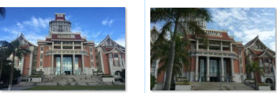
经过RANSAC算法:
3.5 经过RANSAC的SIFT匹配实验小结

对比景深丰富的场景和景深单一的场景,景深丰富的场景匹配到的特征点较多且二者在RANSAC算法上景深单一的场景得到的效果更好也就是最后得到的匹配特征点准确率较高。直接通过SIFT特征提取匹配的结果并不是非常乐观,存在比较多的错误匹配。根据上图可以看出红色圈出部分大本钟顶端的三条连接线的两点明显不是匹配特征点,说明SIFI特征匹配出现了错配,且经过RANSAC算法之后,剔除了大部分的错误匹配点,还存在少数的错误点。接着分析景深单一的实验结果可以看出遮罩物带来了一定的错误匹配,经过RANSAC算法之后这些错误匹配点也没能被剔除。虽然经过RANSAC算法后某些错误匹配仍然存在,误差不可避免,但总体来说,已经达到了非常理想的效果。
四、实验总结和实验遇到的问题
4.1 实验总结
1、SIFT匹配出现匹配错误的点可能是由于对称,加上SIFT具有旋转不变性的特征,所以匹配的都是对称的点,或者是相似度极高的点。
2、对边缘光滑的目标无法准确提取特征点,以及对模糊的图像和边缘平滑的图像,检测出的特征点过少,对圆则是更加难以检测。
3、SIFT特征提取和检索在少数的几个物体也可以产生大量的SIFT特征向量。
4、SIFT算法在一定程度上可解决目标的旋转、缩放、平移,光照变换,目标遮挡带来的影响。
4.2 实验遇到的问题
1、问题:在使用SIFT特征提取和匹配的时候出现empire.sift not found
解决方法:为了计算图像的SIFT特征,需要用到开源工具包VLFeat
把vlfeat文件夹下win64中的sift.exe和vl.dll这两个文件复制到项目的文件夹中。
修改PCV文件夹里面的localdescriptors文件夹中的sift.py文件,修改其中的cmmd内的路径为:cmmd = str(r"D:\PythonWork\SIFT\sift.exe “+imagename+” --output="+resultname+" "+params) (路径是项目文件夹中的sift.exe的路径)
2、问题:在进行检索时,图片格式为png会造成超出范围错误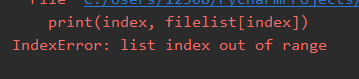
解决:将图片格式改正为jpg即可解决