经典卷积神经网络——AlexNet

概述：

当我们站在2012年的时间节点上，AlexNet网络模型的出现，可以说是CNN的里程碑。由于它将ImageNet LSVRC-2010图片识别测试的错误率从之前最好记录top-1 and top-5 测试集 错误率 47.1% and 28.2% 一下子降低到了 37.5% and 17.0%，虽然它不是CNN的开创者，但它首次使用了很多现代深度卷积神经网络（Deep Convolutional Neural Networks）一些技术，比如使用GPU进行并行训练（当时的旗舰级别GPU只有GTX 580 3GB，对于如此深度的CNN并不足够，因此网络被分成上下两层，一块GPU处理一部分的数据，并在中间部分层进行数据通讯），采用了ReLU作为非线性激活函数，使用Dropout（对于一部分的节点设置一个丢弃的概率 p = 0.5 ，通过将随机训练中的一些节点“暂时丢掉”，如果本次抽中“dropout”，那这个节点就不参与正向和反向的传播计算）来防止过拟合，使用数据增强（Data Augmentation）来提高模型的准确率等，因此它是深度卷积网络热潮的开端，从此以后人们开始更加关注CNN在图像方面的应用，以致后来产生了越来越强大的模型，比如GooLeNet、VGGNet、ResNet、Mask RCNN等等。

原论文链接：https://papers.nips.cc/paper/4824-imagenet-classification-with-deep-convolutional-neural-networks.pdf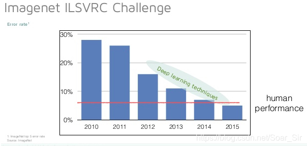

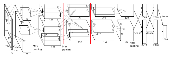
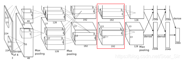
图1. AlexNet赢得了2012年ImageNet图像分类竞赛的冠军

AlexNet结构

AlexNet网络总共有8层构成，其中5层的卷积层（convolutional layers）、3个全连接层（fully connected layers）和1个softmax层。原论文中就是这张图，后来这张图被无数次的引用到各种CNN的课程和会议上。在 ILSVRC-2010中，它能够训练出1.2亿图片模型，其中验证集有：5，000 张图片，测试集有：150，000张图片。虽然这个网络看起来很简单，但是站在2012年那个时间节点上，对于当时的神经网络模型来说已经是一个非常重大的突破了。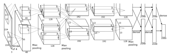

其中每个层的功能组成：

1. 输入层，大小为224 × 224 × 3的图像;
2. 第一个卷积层，使用两个大小为11 × 11 × 3 × 48的卷积核，步长s = 4，零填充p = 3，得到两个大小为55 × 55 × 48的特征映射组。
3. 第一个池化层（汇聚层），使用大小为 3 × 3 的最大汇聚操作，步长 s = 2，得到两个27 × 27 × 48的特征映射组。
4. 第二个卷积层，使用两个大小为5 × 5 × 48 × 128的卷积核，步长s = 1，零填充p = 2，得到两个大小为27 × 27 × 128的特征映射组。

Layer1：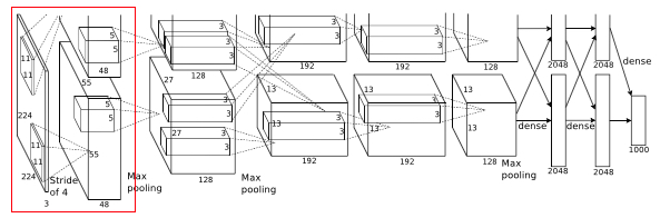

将图像输入到该层之前，训练集中的图片通过重新缩放图像以使得较短边长度为256，然后裁剪出中心256 * 256的固定大小图片。为了防止在该网络上出现过拟合现象，在一些层中dropout的值设定为0.5，并且使用两种保留标签的数据增强方法。 一个是从每个图像中提取随机224 * 224 patch。 因此，该方法通过合理的量增加训练集的大小。 另一种是执行变换以改变图像的照明强度和颜色，因为对象标识对这些图像是不变的。并且使用ReLU（y = max（0, x））作为其激活函数。 通过使用这些神经元，训练时间将根据观察结果减少。

• Then this 224 * 224 * 3 image is given to 1st convolutional layer.
• Where this layer filters the image with 96 kernels of size 11 * 11 * 3
• Stride - 4, assuming padding is 2 Here stride(s) < kernel size(z) (4 < 11), so this overlapping pooling. According to the paper, the models with overlapping pooling find it slightly more difficult to overfit.
• Therefore output = (224 - 11 + 2 *2)/4 + 1 = 55
• Output is of size 55 * 55 * 96
• To this output, local response normalization(LRN) is applied which is a brightness normalization.
• After LRN, max pooling layer is applied where stride is 2 and kernel size is 3 * 3
• Therefore now output is 27((55 - 3)/2 + 1 ) * 27 * 96

Layer2：

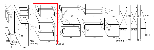
• Input to this layer is 27 * 27 * 96
• Filters = 256
• Kernel size = 5 * 5 * 48, padding = 2
• Stride = 1
• Output width or height = (27 - 5 + 2 * 2)/1 + 1 = 27
• Output is 27 * 27 * 256
• This is followed by LRN and max pooling layer
• Final output layer is
  • Max pooling kernel of size 3 * 3 and stride 1
  • Output width or height = (27 - 3 + 2)/1 + 1 = 27
  • Final output = 27 * 27 * 256

Layer3：

• Input to this layer is 27 * 27 * 256
• Filters = 384
• Kernel size 3 * 3 *256, padding - 1
• Output width or height = (27 - 3 + 2)/1 + 1 = 27
• Final output is 27 * 27 * 384

Layer4：

• Input to this layer is 27 * 27 * 384
• Filters = 384
• Kernel size is 3 * 3 * 192, padding = 1
• Output width or height = (27 - 3 + 2)/1 + 1 = 27
• Final output is 27 * 27 * 384

Layer5：

Similarly after the fifth convolutional layer

• As filters = 256
• Output is 27 * 27 * 256
• After the max pooling layer
  • Kernel size is 3 * 3 and stride 2
  • Final output width or height = (27 - 3 )/2 + 1 = 13
  • Final output is 13 * 13 * 256 And other two layers are fully connected layers of 4096 each

Softmax：

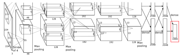
To the final layer 1000 way softmax is used to get predicted probabilities for each class.

代码实现（pytorch）：

import torch.nn as nn
from .utils import load_state_dict_from_url


__all__ = ['AlexNet', 'alexnet']


model_urls = {
    'alexnet': 'https://download.pytorch.org/models/alexnet-owt-4df8aa71.pth',
}


class AlexNet(nn.Module):

    def __init__(self, num_classes=1000):
        super(AlexNet, self).__init__()
        self.features = nn.Sequential(
            nn.Conv2d(3, 64, kernel_size=11, stride=4, padding=2),
            nn.ReLU(inplace=True),
            nn.MaxPool2d(kernel_size=3, stride=2),
            nn.Conv2d(64, 192, kernel_size=5, padding=2),
            nn.ReLU(inplace=True),
            nn.MaxPool2d(kernel_size=3, stride=2),
            nn.Conv2d(192, 384, kernel_size=3, padding=1),
            nn.ReLU(inplace=True),
            nn.Conv2d(384, 256, kernel_size=3, padding=1),
            nn.ReLU(inplace=True),
            nn.Conv2d(256, 256, kernel_size=3, padding=1),
            nn.ReLU(inplace=True),
            nn.MaxPool2d(kernel_size=3, stride=2),
        )
        self.avgpool = nn.AdaptiveAvgPool2d((6, 6))
        self.classifier = nn.Sequential(
            nn.Dropout(),
            nn.Linear(256 * 6 * 6, 4096),
            nn.ReLU(inplace=True),
            nn.Dropout(),
            nn.Linear(4096, 4096),
            nn.ReLU(inplace=True),
            nn.Linear(4096, num_classes),
        )

    def forward(self, x):
        x = self.features(x)
        x = self.avgpool(x)
        x = x.view(x.size(0), 256 * 6 * 6)
        x = self.classifier(x)
        return x