python实现PCA降维及可视化

实现功能：

python对数据清洗以及数据编码（具体实现方式可查看前两篇文章）后的变量进行PCA降维，并进行可视化展示。

实现代码：

# 导入需要的库
import numpy as np
import pandas as pd
import seaborn as sns
from sklearn import preprocessing
import matplotlib.pyplot as plt
from sklearn.decomposition import PCA

def Read_data(file):
    dt = pd.read_csv(file)
    dt.columns = ['age', 'sex', 'chest_pain_type', 'resting_blood_pressure', 'cholesterol',
                  'fasting_blood_sugar', 'rest_ecg', 'max_heart_rate_achieved','exercise_induced_angina',
                  'st_depression', 'st_slope', 'num_major_vessels', 'thalassemia', 'target']
    data =dt
    pd.set_option('display.max_rows', None)
    pd.set_option('display.max_columns', None)
    pd.set_option('display.width', None)
    pd.set_option('display.unicode.ambiguous_as_wide', True)
    pd.set_option('display.unicode.east_asian_width', True)
    print(data.head())
    return data

def data_clean(data):
    # 数据清洗
    # 重复值处理
    print('存在' if any(data.duplicated()) else '不存在', '重复观测值')
    data.drop_duplicates()

    # 缺失值处理
    # print(data.isnull())
    # print(data.isnull().sum())   #检测每列中缺失值的数量
    # print(data.isnull().T.sum())    #检测每行缺失值的数量
    print('不存在' if any(data.isnull()) else '存在', '缺失值')
    data.dropna()  # 直接删除记录
    data.fillna(method='ffill')  # 前向填充
    data.fillna(method='bfill')  # 后向填充
    data.fillna(value=2)  # 值填充
    data.fillna(value={'resting_blood_pressure': data['resting_blood_pressure'].mean()})  # 统计值填充

    # 异常值处理
    data1 = data['resting_blood_pressure']
    # 标准差监测
    xmean = data1.mean()
    xstd = data1.std()
    print('存在' if any(data1 > xmean + 2 * xstd) else '不存在', '上限异常值')
    print('存在' if any(data1 < xmean - 2 * xstd) else '不存在', '下限异常值')
    # 箱线图监测
    q1 = data1.quantile(0.25)
    q3 = data1.quantile(0.75)
    up = q3 + 1.5 * (q3 - q1)
    dw = q1 - 1.5 * (q3 - q1)
    print('存在' if any(data1 > up) else '不存在', '上限异常值')
    print('存在' if any(data1 < dw) else '不存在', '下限异常值')
    data1[data1 > up] = data1[data1 < up].max()
    data1[data1 < dw] = data1[data1 > dw].min()
    # print(data1)
    return data


def data_encoding(data):
    #========================数据编码===========================
    data = data[["age", 'sex', "chest_pain_type", "resting_blood_pressure", "cholesterol",
                 "fasting_blood_sugar", "rest_ecg","max_heart_rate_achieved", "exercise_induced_angina",
                 "st_depression", "st_slope", "num_major_vessels","thalassemia","target"]]
    Discretefeature=['sex',"chest_pain_type", "fasting_blood_sugar", "rest_ecg",
          "exercise_induced_angina",  "st_slope", "thalassemia"]
    Continuousfeature=["age", "resting_blood_pressure", "cholesterol",
                       "max_heart_rate_achieved","st_depression","num_major_vessels"]

    df = pd.get_dummies(data,columns=Discretefeature)
    print(df.head())

    df[Continuousfeature]=(df[Continuousfeature]-df[Continuousfeature].mean())/(df[Continuousfeature].std())
    print(df.head())
    df["target"]=data[["target"]]
    print(df)
    return df

def PCA_analysis(data):
    # X提取变量特征；Y提取目标变量
    X = data.drop('target', axis=1)
    y = data['target']
    pca = PCA(n_components=2)

    reduced_x = pca.fit_transform(X)  # 得到了pca降到2维的数据
    print(reduced_x.shape)
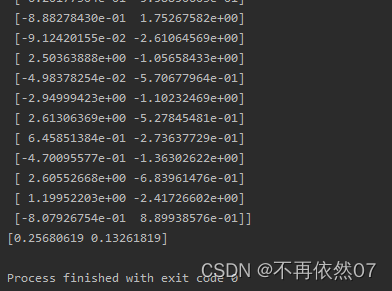
    print(reduced_x)

    yes_x, yes_y = [], []
    no_x, no_y = [], []

    for i in range(len(reduced_x)):
        if y[i] == 1:
            yes_x.append(reduced_x[i][0])
            yes_y.append(reduced_x[i][1])
        elif y[i] == 0:
            no_x.append(reduced_x[i][0])
            no_y.append(reduced_x[i][1])

    font = {'family': 'Times New Roman',
            'size': 16,
            }
    sns.set(font_scale=1.2)

    plt.rc('font',family='Times New Roman')
    plt.scatter(yes_x, yes_y, c='r', marker='o',label='Yes')
    plt.scatter(no_x, no_y, c='b', marker='x',label='No')
    plt.title("PCA analysis")  # 显示标题
    plt.legend()
    plt.show()
    print(pca.explained_variance_ratio_)  # 输出贡献率


if __name__=="__main__":
    data1=Read_data("F:\数据杂坛\\0504\heartdisease\Heart-Disease-Data-Set-main\\UCI Heart Disease Dataset.csv")
    data1=data_clean(data1)
    data2=data_encoding(data1)
    PCA_analysis(data2)

实现效果：

喜欢记得点赞，在看，收藏，

关注V订阅号：数据杂坛，获取完整代码和效果，将持续更新！