文章目录
Lecture 5: Training versus Testing
Recap and Preview
Two Central Questions
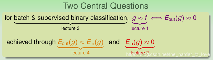
make sure that E o u t ( g ) E_{out} (g)Eout(g) is close enough to E i n ( g ) E_{in} (g)Ein(g).
make E i n ( g ) E_{in} (g)Ein(g)mall enough.
Fun Time
Data size: how large do we need?
One way to use the inequality
P [ ∣ E in ( g ) − E out ( g ) ∣ > ϵ ] ≤ 2 ⋅ M ⋅ exp ( − 2 ϵ 2 N ) ⎵ δ \mathbb{P}\left[ | E_{\text { in }}(g)-E_{\text { out }}(g) |>\epsilon\right] \leq \underbrace{2 \cdot M \cdot \exp \left(-2 \epsilon^{2} N\right)}_{\delta}P[∣E in (g)−E out (g)∣>ϵ]≤δ2⋅M⋅exp(−2ϵ2N)
is to pick a tolerable difference ? as well as a tolerable BAD probability δ, and then gather data with size (N) large enough to achieve those tolerance criteria. Let ? = 0.1, δ = 0.05, and M = 100.
What is the data size needed?
1. 215 2. 415 ✓ \checkmark✓ 3. 615 4. 815
Explanation
N = 1 2 ϵ 2 ln 2 M δ N=\frac{1}{2 \epsilon^{2}} \ln \frac{2 M}{\delta}N=2ϵ21lnδ2M
所以N = 414.7 ≈ 415 N =414.7 \approx 415N=414.7≈415
Effective Number of Lines
Uniform Bound
B m : ∣ E in ( h m ) − E out ( h m ) ∣ > ϵ B_{m} : | E_{\text { in }}\left(h_{m}\right)-E_{\text { out }}\left(h_{m}\right) |>\epsilonBm:∣E in (hm)−E out (hm)∣>ϵ
for most D DD,E i n ( h i ) = E i n ( h j ) E_{\mathrm{in}}(h_i) = E_{\mathrm{in}}(h_j)Ein(hi)=Ein(hj)
E o u t ( h i ) ≈ E o u t ( h j ) E_{\mathrm{out}}(h_i) \approx E_{\mathrm{out}}(h_j)Eout(hi)≈Eout(hj)
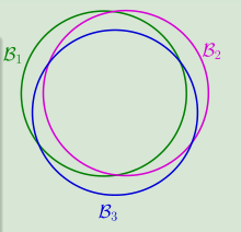
P D [ B A D D f o r h 1 ] + P D [ B A D D f o r h 2 ] + . . . + P D [ B A D D f o r h M ] ( u n i o n b o u n d ) \begin{aligned}\mathbb{P}_{\mathcal{D}}[\mathrm{BAD} \ \mathcal{D} \ for \ h_1]+\mathbb{P}_{\mathcal{D}}[\mathrm{BAD} \ \mathcal{D} \ for \ h_2]+...+\mathbb{P}_{\mathcal{D}}[\mathrm{BAD} \ \mathcal{D} \ for \ h_M](union \ bound)\end{aligned}PD[BAD D for h1]+PD[BAD D for h2]+...+PD[BAD D for hM](union bound) over-estimating
为了合并重叠的部分,我们按照类别将类似的假设分组归类。
Many Lines
H = { all lines in R 2 } \mathcal{H}=\left\{\text { all lines in } \mathbb{R}^{2}\right\}H={ all lines in R2}
Effective Number of Hypotheses
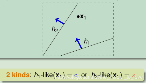
1点2个类别
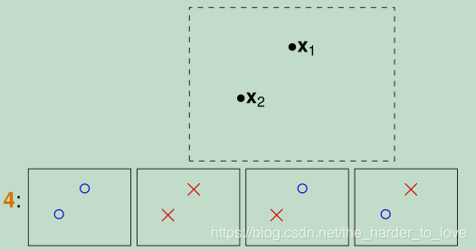
2个点4个类别
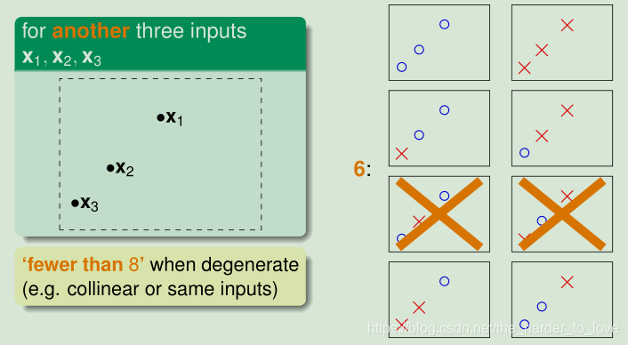
3个点6个类别
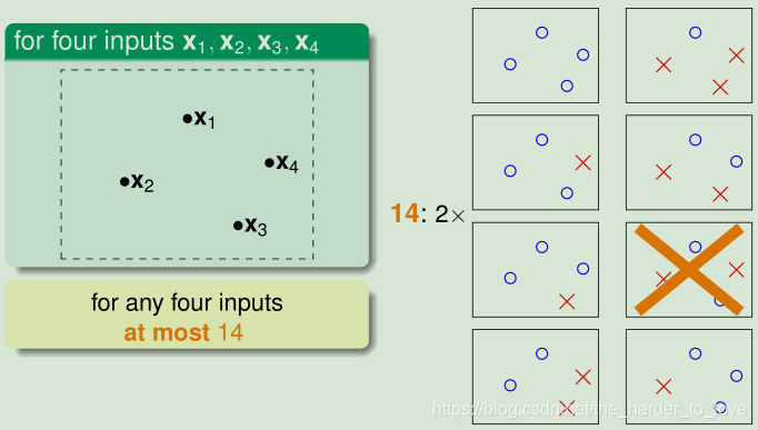
4个点14个类别
e f f e c t i v e ( N ) < < 2 N effective(N)<< 2^Neffective(N)<<2N,用有效类别数(e f f e c t i v e ( N ) effective(N)effective(N))替换M MM(infite)
Fun Time
What is the effective number of lines for five inputs $ \in R^2$ ?
1. 14 2. 16 3. 22 ✓ \checkmark✓ 4. 32
Explanation
总共有32(2 5 2^525)种
5个O:1种,4个O1个X:5种,3个O2个X:共有$C_5^3$10种,只有5种满足条件。
而又O和X等价
所以有效类别数共有2X(1+5+5)=22种。
Growth Function
e f f e c t i v e ( N ) < < 2 N effective(N)<< 2^Neffective(N)<<2N
M ⇒ e f f e c t i v e ( N ) M \Rightarrow effective(N)M⇒effective(N)
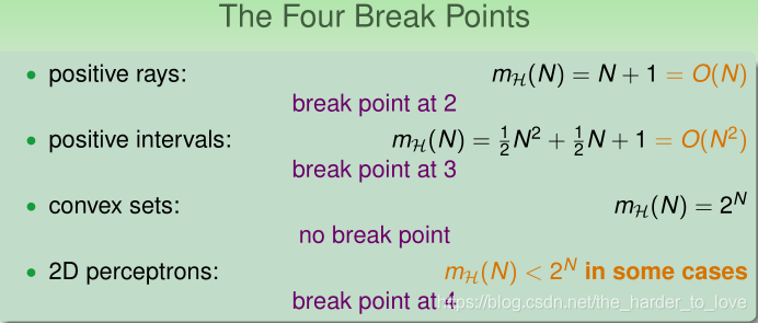
Growth Function for Positive Rays
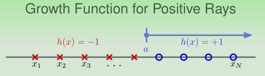
h ( x ) = sign ( x − a ) m H ( N ) = N + 1 ≪ 2 N h(x)=\operatorname{sign}(x-a) \\ m_{\mathcal{H}}(N)=N+1 \ll 2^{N}h(x)=sign(x−a)mH(N)=N+1≪2N
Growth Function for Positive Intervals
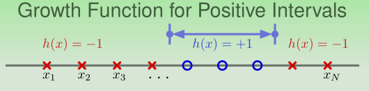
h ( x ) = + 1 if x ∈ [ ℓ , r ) , − 1 o t h e r w i s e m H ( N ) = 1 2 N 2 + 1 2 N + 1 ≪ 2 N h(x)=+1 \text { if } x \in[\ell, r),-1 \ otherwise \\ m_{\mathcal{H}}(N)=\frac{1}{2} N^{2}+\frac{1}{2} N+1 \ll 2^{N}h(x)=+1 if x∈[ℓ,r),−1 otherwisemH(N)=21N2+21N+1≪2N
Growth Function for Convex Sets

e v e r y d i c h o t o m y c a n b e i m p l e m e n t e d m H ( N ) = 2 N every \ dichotomy \ can \ be \ implemented \\ m_{\mathcal{H}}(N)=2^{N}every dichotomy can be implementedmH(N)=2N
m H ( N ) = 2 N m_{\mathcal{H}}(N)=2^{N}mH(N)=2N call those N NN inputs ‘shattered’ by H HH
Fun Time
Consider positive and negative rays as H, which is equivalent to the perceptron hypothesis set in 1D. The hypothesis set is often called ‘decision stump’ to describe the shape of its hypotheses. What is the growth function m H ( N ) m_H (N)mH(N)?
1. N 2. N+1 3. 2N ✓ \checkmark✓ 4. 2 N 2^N2N
Explanation
正或负方向的Positive Intervals,再加上全X和全O。
2X(N-1)+2 = 2N
Break Point
m H m_{\mathcal{H}}mH是多项式(O ( N k − 1 ) O\left(N^{k-1}\right)O(Nk−1)),我们用它替换M MM
m H ( k ) < 2 k m_{\mathcal{H}}(k)<2^{k}mH(k)<2k call k a break point for H HH
if k is a break point, k+1, k+2, k+3,… also break points! k is the minimum break point.
Fun Time
Consider positive and negative rays as H, which is equivalent to the perceptron hypothesis set in 1D. As discussed in an earlier quiz question, the growth function m H ( N ) = 2 N m_H (N) = 2NmH(N)=2N. What is the minimum break point for H HH?
1. 1 2. 2 3. 3 ✓ \checkmark✓ 4. 4
Explanation
m H ( N ) = 2 N 2 ∗ 2 = 4 = 2 2 , 2 ∗ 3 = 6 < 2 3 m_H (N) = 2N \\ 2*2 = 4 = 2^2, \quad 2*3 = 6 < 2^3mH(N)=2N2∗2=4=22,2∗3=6<23
正负线的"一线曙光"是3.
Summary
讲义总结
m H m_{\mathcal{H}}mH是多项式(O ( N k − 1 ) O\left(N^{k-1}\right)O(Nk−1)),我们用它替换M MM,降低假设集的上界。
通过minimum break point,求出多项式的幂级数。
Recap and Preview
two questions: E o u t ( g ) ≈ E i n ( g ) E_{out} (g) ≈ E_{in} (g)Eout(g)≈Ein(g), and E i n ( g ) ≈ 0 E_{in} (g) ≈ 0Ein(g)≈0
Effective Number of Lines
at most 14 through the eye of 4 inputs
Effective Number of Hypotheses
at most m H ( N ) m_H (N)mH(N) through the eye of N NN inputs
Break Point
when m H ( N ) m_H (N)mH(N) becomes ‘non-exponential’
参考文献
《Machine Learning Foundations》(机器学习基石)—— Hsuan-Tien Lin (林轩田)