MATLAB实现一个EKF-2D-SLAM（已开源）

1. SLAM问题定义

同时定位与建图（SLAM）的本质是一个估计问题，它要求移动机器人利用传感器信息实时地对外界环境结构进行估计，并且估算出自己在这个环境中的位置，Smith 和Cheeseman在上个世纪首次将EKF估计方法应用到SLAM。

以滤波为主的SLAM模型主要包括三个方程：

1）运动方程：它会增加机器人定位的不确定性

2）根据观测对路标初始化的方程：它根据观测信息，对新的状态量初始化。

3）路标状态对观测的投影方程：根据观测信息，对状态更新，纠正，减小不确定度。

2. EKF-SLAM维护的数据地图

系统状态x是一个很大的向量，它包括机器人的状态和路标点的状态，

$$\mathbf{x}=\left[\begin{array}{c}\mathcal{R}\\ \mathcal{M}\end{array}\right]=\left[\begin{array}{c}\mathcal{R}\\ {\mathcal{L}}_1\\ ⋮\\ {\mathcal{L}}_n\end{array}\right]$$
其中$\mathcal{R}$是机器人状态，$\mathcal{M}=\left({\mathcal{L}}_1，\dots ，{\mathcal{L}}_n\right)$是n个当前已经观测过的路标点状态集合。

在EKF中，x被认为服从高斯分布，所以，EKF-SLAM的地图被建模为x的均值$\overline{x}$与协方差$\mathbf{P}$,

$$\overline{\mathbf{x}}=\left[\frac{\overline{\mathcal{R}}}{\mathcal{M}}\right]=\left[\begin{array}{c}\overline{\mathcal{R}}\\ {\overline{\mathcal{L}}}_1\\ ⋮\\ {\overline{\mathcal{L}}}_n\end{array}\right]\mathbf{P}=\left[\begin{array}{cc}{\mathbf{P}}_{\mathcal{R}\mathcal{R}}& {\mathbf{P}}_{\mathcal{R}\mathcal{M}}\\ {\mathbf{P}}_{\mathcal{M}\mathcal{R}}& {\mathbf{P}}_{\mathcal{M}\mathcal{M}}\end{array}\right]=\left[\begin{array}{cccc}{\mathbf{P}}_{\mathcal{R}\mathcal{R}}& {\mathbf{P}}_{\mathcal{R}{\mathcal{L}}_1}& \cdots & {\mathbf{P}}_{\mathcal{R}{\mathcal{L}}_n}\\ {\mathbf{P}}_{{\mathcal{L}}_1\mathcal{R}}& {\mathbf{P}}_{{\mathcal{L}}_1{\mathcal{L}}_1}& \cdots & {\mathbf{P}}_{{\mathcal{L}}_n}{\mathcal{L}}_n\\ ⋮& ⋮& \ddots & ⋮\\ {\mathbf{P}}_{{\mathcal{L}}_n\mathcal{R}}& {\mathbf{P}}_{{\mathcal{L}}_n{\mathcal{L}}_1}& \cdots & {\mathbf{P}}_{{\mathcal{L}}_n{\mathcal{L}}_n}\end{array}\right]$$
因此EKF-SLAM的目标就是根据运动模型和观测模型及时更新地图量$\left\{\overline{\mathbf{x}},\mathbf{P}\right\}$

3. EKF-SLAM算法实施

3.1 地图初始化

显而易见，在机器人开始之前是没有任何路标点的信息的，因此此时地图中只有机器人自己的状态信息，因此$n=0,x=\mathcal{R}$。SLAM中经常把机器人初始位姿认为是地图的原点，其初始协方差可以按实际情况设定，比如：

$$\overline{\mathbf{x}}=\left[\begin{array}{l}x\\ y\\ \theta \end{array}\right]=\left[\begin{array}{l}0\\ 0\\ 0\end{array}\right]\mathbf{P}=\left[\begin{array}{lll}0& 0& 0\\ 0& 0& 0\\ 0& 0& 0\end{array}\right]$$

3.2 运动模型

在EKF中如果x是状态量，u是控制输入，n是噪声变量，那么我们可以得到一般的状态更新函数：

$$\mathbf{x}\leftarrow f(\mathbf{x},\mathbf{u},\mathbf{n})$$

EKF的预测步骤为：

$$\begin{array}{l}\overline{\mathbf{x}}\leftarrow f(\overline{\mathbf{x}},\mathbf{u},0)\\ \mathbf{P}\leftarrow {\mathbf{F}}_{\mathbf{x}}\mathbf{P}{\mathbf{F}}_{\mathbf{x}}^{\top }+{\mathbf{F}}_{\mathbf{n}}\mathbf{N}{\mathbf{F}}_{\mathbf{n}}^{\top }\end{array}$$

其中雅克比矩阵${\mathbf{F}}_{\mathbf{x}}=\frac{\partial f(\overline{\mathbf{x}},\mathbf{u})}{\partial \mathbf{x}}$，${\mathbf{F}}_{\mathbf{n}}=\frac{\partial f(\overline{\mathbf{x}},\mathbf{u})}{\partial \mathbf{n}}$，$\mathbf{N}$是随机变量n的协方差。

但是在EKF-SLAM中，只有一部分状态$\mathcal{R}$是随运动而改变的，其余所有路标状态不改变，所以SLAM的运动方程为：

$$\begin{array}{l}\mathcal{R}\leftarrow f_{\mathcal{R}}(\mathcal{R},\mathbf{u},\mathbf{n})\\ \mathcal{M}\leftarrow \mathcal{M}\end{array}$$

因此我们可以得到稀疏的雅克比矩阵：

$${\mathbf{F}}_{\mathbf{x}}=\left[\begin{array}{cc}\frac{\partial f_{\mathcal{R}}}{\partial \mathcal{R}}& 0\\ 0& \mathbf{I}\end{array}\right]{\mathbf{F}}_{\mathbf{n}}=\left[\begin{array}{c}\frac{\partial f_{\mathcal{R}}}{\partial \mathbf{n}}\\ 0\end{array}\right]$$

最终我们得到了用于运动模型的EKF稀疏预测公式

$$\overline{\mathcal{R}}\leftarrow f_{\mathcal{R}}(\overline{\mathcal{R}},\mathbf{u},0)$$

$${\mathbf{P}}_{\mathcal{R}\mathcal{R}}\leftarrow \frac{\partial f_{\mathcal{R}}}{\partial \mathcal{R}}{\mathbf{P}}_{\mathcal{R}\mathcal{R}}\frac{\partial f_{\mathcal{R}}^T}{\partial \mathcal{R}}+\frac{\partial f_{\mathcal{R}}}{\partial \mathbf{n}}\mathbf{N}\frac{\partial f_{\mathcal{R}}^T}{\partial \mathbf{n}}$$

$${\mathbf{P}}_{\mathcal{R}\mathcal{M}}\leftarrow \frac{\partial f_{\mathcal{R}}}{\partial \mathcal{R}}{\mathbf{P}}_{\mathcal{R}\mathcal{M}}$$

$${\mathbf{P}}_{\mathcal{M}\mathcal{R}}\leftarrow {\mathbf{P}}_{\mathcal{R}\mathcal{M}}^{\top }$$

3.3 已经加入地图的状态量观测更新

在EKF中，我们有以下一般的观测方程

$$\mathbf{y}=h(\mathbf{x})+\mathbf{v}$$

其中$\mathbf{y}$是测量噪声，$\mathbf{x}$是全状态，$h()$是观测函数，$v$是测量噪声。

典型的EKF观测更新为：

$$\overline{\mathbf{z}}=\mathbf{y}-h(\overline{\mathbf{x}})$$

$$\mathbf{Z}={\mathbf{H}}_{\mathbf{x}}\mathbf{P}{\mathbf{H}}_{\mathbf{x}}^{\top }+\mathbf{R}$$

$$\mathbf{K}=\mathbf{P}{\mathbf{H}}_{\mathbf{x}}^{\top }{\mathbf{Z}}^{-1}$$

$$\overline{\mathbf{x}}\leftarrow \overline{\mathbf{x}}+\mathbf{K}\overline{\mathbf{z}}$$

$$\mathbf{P}\leftarrow \mathbf{P}-\mathbf{K}\mathbf{Z}{\mathbf{K}}^{\top }$$

雅克比矩阵${\mathbf{H}}_{\mathbf{x}}=\frac{\partial h(\overline{\mathbf{x}})}{\partial \mathbf{x}}$，$\mathbf{R}$是测量噪声的协方差矩阵。

在SLAM中，观测指的是机器人上的传感器观测到某些路标点，并对路标点进行参数化的输出。每次可能对路标点有多个观测值，这里每使用一个观测值，就进行一次状态更新。

观测的结果依赖于机器人的状态$\mathcal{R}$,传感器的状态$\mathcal{S}$和路标点的状态${\mathcal{L}}_i$，并且这里假设，传感器的状态与机器人的状态差了一个固定的坐标变化，其实也就是外参固定。当观测到路标点$i$时，可以得到如下关系：
$${\mathbf{y}}_i=h_i\left(\mathcal{R},\mathcal{S},{\mathcal{L}}_i\right)+\mathbf{v}$$

这就是观测方程，它不依赖于除了${\mathcal{L}}_i$外的任何路标点状态。因此EKF-SLAM的雅克比${\mathbf{H}}_{\mathbf{x}}$也是稀疏的：

$${\mathbf{H}}_{\mathbf{x}}=\left[\begin{array}{llllllll}{\mathbf{H}}_{\mathcal{R}}& 0& \cdots & 0& {\mathbf{H}}_{{\mathcal{L}}_i}& 0& \cdots & 0\end{array}\right]$$

其中${\mathbf{H}}_{\mathcal{R}}=\frac{\partial h_i\left(\overline{\mathcal{R}},\mathcal{S},{\overline{\mathcal{L}}}_i\right)}{\partial \mathcal{R}}$，${\mathbf{H}}_{{\mathcal{L}}_i}=\frac{\partial h_i\left(\overline{\mathcal{R}},\mathcal{S},{\overline{\mathcal{L}}}_i\right)}{\partial {\mathcal{L}}_i}$。由于这里的稀疏性，EKF-SLAM的观测更新变成：

$$\overline{\mathbf{z}}={\mathbf{y}}_i-h_i\left(\overline{\mathcal{R}},\mathcal{S},{\overline{\mathcal{L}}}_i\right)$$

$$\mathbf{Z}=\left[\begin{array}{cc}{\mathbf{H}}_{\mathcal{R}}& {\mathbf{H}}_{{\mathcal{L}}_i}\end{array}\right]\left[\begin{array}{cc}{\mathbf{P}}_{\mathcal{R}\mathcal{R}}& {\mathbf{P}}_{\mathcal{R}{\mathcal{L}}_i}\\ {\mathbf{P}}_{{\mathcal{L}}_i\mathcal{R}}& {\mathbf{P}}_{{\mathcal{L}}_i{\mathcal{L}}_i}\end{array}\right]\left[\begin{array}{c}{\mathbf{H}}_{\mathcal{R}}^{\top }\\ {\mathbf{H}}_{{\mathcal{L}}_i}^{\top }\end{array}\right]+\mathbf{R}$$

$$\mathbf{K}=\left[\begin{array}{ll}{\mathbf{P}}_{\mathcal{R}\mathcal{R}}& {\mathbf{P}}_{\mathcal{R}{\mathcal{L}}_i}\\ {\mathbf{P}}_{\mathcal{M}\mathcal{R}}& {\mathbf{P}}_{\mathcal{M}{\mathcal{L}}_i}\end{array}\right]\left[\begin{array}{l}{\mathbf{H}}_{\mathcal{R}}^{\top }\\ {\mathbf{H}}_{{\mathcal{L}}_i}^{\top }\end{array}\right]{\mathbf{Z}}^{-1}$$

$$\overline{\mathbf{x}}\leftarrow \overline{\mathbf{x}}+\mathbf{K}\overline{\mathbf{z}}$$

$$\mathbf{P}\leftarrow \mathbf{P}-\mathbf{K}\mathbf{Z}{\mathbf{K}}^{\top }$$

3.4 观测方程可逆时的状态增广

这里的状态增广指的是新发现的路标点的初始化。当机器人发现了曾经未观测到的路标点时，会利用观测方程将新的路标状态加入地图，这一步操作会增大总状态向量的大小。可以看到EKF-SLAM中的滤波器大小动态变化的。

当传感器信息可以提供新发现路标点的所有自由度，也就是观测方程是双射时，只需要根据观测方程$h()$的逆运算，即可以得到机器人状态$\mathcal{R}$，传感器状态$\mathcal{S}$，观测量${\mathbf{y}}_{n+1}$，观测噪声$v$，它们与新路标点状态的关系：

$${\mathcal{L}}_{n+1}=g\left(\mathcal{R},\mathcal{S},{\mathbf{y}}_{n+1},v\right)$$

上式是单个路标点的逆观测模型。

路标点的均值和雅克比：

$${\overline{\mathcal{L}}}_{n+1}=g\left(\overline{\mathcal{R}},\mathcal{S},{\mathbf{y}}_{n+1},0\right)$$

$${\mathbf{G}}_{\mathcal{R}}=\frac{\partial g\left(\overline{\mathcal{R}},\mathcal{S},{\mathbf{y}}_{n+1},0\right)}{\partial \mathcal{R}}$$

$${\mathbf{G}}_{\mathbf{v}}=\frac{\partial g\left(\overline{\mathcal{R}},\mathcal{S},{\mathbf{y}}_{n+1},0\right)}{\partial \mathbf{v}}$$

显然，新加路标点状态的协方差${\mathbf{P}}_{\mathcal{L}\mathcal{L}}$，以及该状态与地图其它状态的互协方差为：

$${\mathbf{P}}_{\mathcal{L}\mathcal{L}}={\mathbf{G}}_{\mathcal{R}}{\mathbf{P}}_{\mathcal{R}\mathcal{R}}{\mathbf{G}}_{\mathcal{R}}^{\top }+{\mathbf{G}}_{\mathbf{v}}\mathbf{R}{\mathbf{G}}_{\mathbf{v}}^{\top }$$

$${\mathbf{P}}_{\mathcal{L}\mathbf{x}}={\mathbf{G}}_{\mathcal{R}}{\mathbf{P}}_{\mathcal{R}\mathbf{x}}={\mathbf{G}}_{\mathcal{R}}\left[\begin{array}{cc}{\mathbf{P}}_{\mathcal{R}\mathcal{R}}& {\mathbf{P}}_{\mathcal{R}\mathcal{M}}\end{array}\right]$$

然后将这些结果加入到地图中，可以得到总状态的均值与协方差矩阵：
$$\overline{\mathbf{x}}\leftarrow \left[\begin{array}{c}\overline{\mathbf{x}}\\ {\overline{\mathcal{L}}}_{n+1}\end{array}\right]$$

$$\mathbf{P}\leftarrow \left[\begin{array}{cc}\mathbf{P}& {\mathbf{P}}_{\mathcal{L}\mathbf{x}}^{\top }\\ {\mathbf{P}}_{\mathcal{L}\mathbf{x}}& {\mathbf{P}}_{\mathcal{L}\mathcal{L}}\end{array}\right]$$

4. 仿真实验

4.1 模型设置

4.1.1 传感器模型

传感器是一个360度的雷达，可以探测发现周围一定范围内的路标点及其类型，其探测半径为r，其观测值为($\xi$，s)。$\xi$为在当前雷达坐标系中路标点与x轴的的夹角，s为路标点与当前雷达坐标系原点的距离。

4.1.2 运动模型

将当前时刻雷达局部坐标系中的（$u_1$,0）点作为下一时刻雷达的位置，所以运动方程可以设为：

$$\left[\begin{array}{c}{x}_n\\ y_n\end{array}\right]=\left[\begin{array}{cc}cos{\theta }_{n-1}& -sin{\theta }_{n-1}\\ sin{\theta }_{n-1}& cos{\theta }_{n-1}\end{array}\right]\left[\begin{array}{c}{u}_1\\ 0\end{array}\right]+\left[\begin{array}{c}{x}_{n-1}\\ y_{n-1}\end{array}\right]+\left[\begin{array}{c}{n}_1\\ 0\end{array}\right]$$

其方位每次增加固定的$u_2$:

$${\theta }_{n+1}={\theta }_n+u_2+n_2$$

其中$n_1,n_2$为系统噪声。

4.1.3 观测模型

设路标点$i$的状态为$x_{L_i}=$($m_1$，$m_2$)，则其在当前雷达坐标系的坐标为：

$$\left[\begin{array}{c}{ladar}_1\\ {ladar}_2\end{array}\right]={\left[\begin{array}{cc}cos{\theta }_n& -sin{\theta }_n\\ sin{\theta }_n& cos{\theta }_n\end{array}\right]}^{-1}\left[\begin{array}{c}{m}_1\\ m_2\end{array}\right]-\left[\begin{array}{c}{x}_n\\ y_n\end{array}\right]$$
则观测量为：

$$\xi =atan2\left({ladar}_2,{ladar}_1\right)+v_1$$

$$s=\sqrt{{\left({ladar}_1\right)}^2+{\left({ladar}_2\right)}^2}+v_2$$

其中$v_1,v_2$为测量噪声。

4.2 实验结果

使用MATLAB编写程序进行仿真。

代码地址:https://github.com/liuzhenboo/EKF-2D-SLAM

4.2.1 第一次状态增广

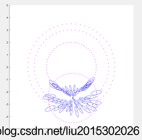
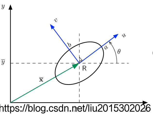
其中左图黑色的点表示滤波器新加入的路标点状态均值，绿色椭圆表征路标状态的协方差，其椭圆方程为：

$$(\mathbf{x}-\overline{\mathbf{x}}{)}^{\top }{\mathbf{P}}^{-1}(\mathbf{x}-\overline{\mathbf{x}})=\text{ const }$$

其中x为路标状态,P为路标的协方差。

程序中是对P进行SVD分解，得到椭圆的方向R以及半轴到的长度，进行绘图。

4.2.2 状态增广，观测更新

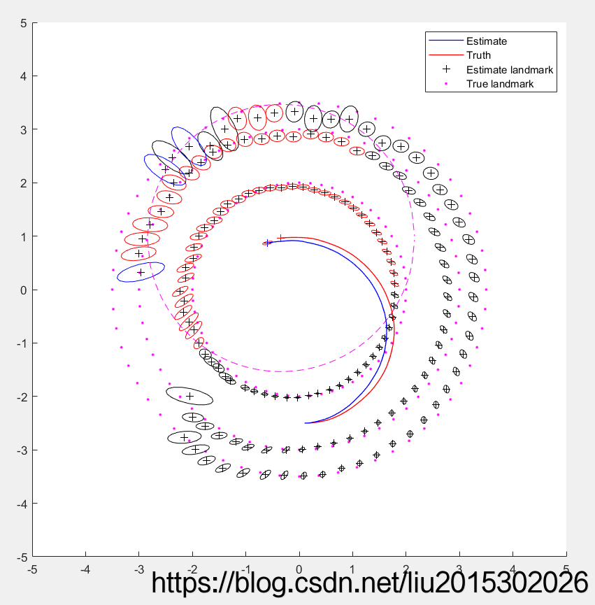
如上图，黑色椭圆对应的路标点表示雷达曾经观测过它，但是当前时刻没有观测到；红色椭圆对应的路标点表示雷达曾经观测过它，并且当前时刻也观测到了；蓝色代表当前刚刚初始化的新路标点。

注意：由于数值计算的原因，图中几何元素的位置关系可能和实际有些许差别；比如有的路标点明明不在雷达范围内，却开始初始化（绿色），这是因为计算过程中matlab四舍五入导致的结果。

4.2.3 状态不再增广，只有观测更新

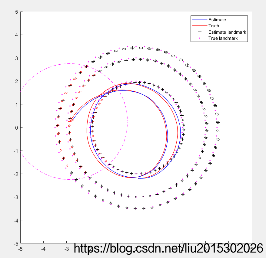
如上图，不再存在蓝色的协方差椭圆，代表状态增广停止，滤波器的大小不再改变。