前面两章主要是下面这两段代码

# 二分法排序
def binary_search(list, item, message):
    low = 0
    high = len(list) - 1

    while low <= high:
        mid = (low + high) // 2
        guess = list[mid]
        print(message + str(mid))
        if guess == item:
            return mid
        if guess > item:
            high = mid - 1
        else:
            low = mid + 1
            return None


my_list = [1, 3, 5, 7, 9]

print(binary_search(my_list, 3, "第一个"))
print(binary_search(my_list, -1, "第二个"))


# 选择排序
def findSmallest(arr):
    smallest = arr[0]
    smallest_index = 0
    for i in range(1, len(arr)):
        if arr[i] < smallest:
            smallest = arr[i]
            smallest_index = i
    return smallest_index

def selectionSort(arr):
    newArr = []
    for i in range(len(arr)):
        smallest = findSmallest(arr)
        newArr.append(arr.pop(smallest))
    return newArr

print(selectionSort([5, 3, 6, 3, 10]))

第三章

递归

编写递归函数时，必须告诉它何时停止递归。因此，每个函数都有两部分：基线条件和递归条件。递归条件指的是函数调用自己，而基线条件指的是函数不再调用自己，从而避免形成无限循环。

栈

两个操作：压入（插入）和弹出（删除并读取）

def greet(name):
	print("hello, " + name + "!")
	greet2(name)
	print("getting ready to say bye...")
	bye()

def greet2(name):
	print("how are you, " + name + "?")

def bye():
	print("ok bye")

当函数被调用时，计算机便会为该函数调用分配一块内存，并将函数涉及的所有变量的值存储到内存中。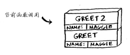

计算机使用一个栈来表示这些内存块，其中第二个内存块位于第一个内存块上面，打印结束后，从函数调用返回。此时，栈顶的内存块被弹出。

现在栈顶的内存块是函数greet的，这意味着返回到了函数greet。当调用函数greet2时，函数greet只执行了一部分，其所有变量值还都在内存里。执行完函数greet2后，回到函数greet，会接着向下执行，再调用函数bye。

打印ok bye结束之后，从函数bye返回，又回到了函数greet，由于没有别的事情做，就从greet返回，这个栈用于存储多个函数的变量，被称作调用栈，所有函数调用都进入调用栈，调用栈很长将会占用大量内存。

第四章 快速排序

分而治之

（1） 找出简单的基线条件
（2） 确定如何缩小问题的规模，使其符合基线条件
给定一个数组[2, 4, 6]，使用递归函数，将这些数字相加，并返回结果。
第一步，找出基线条件，如果数组不包含任何元素或只包含一个元素，计算总和将很容易。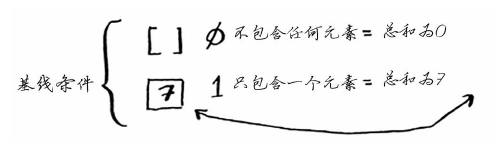

第二步，每次递归调用都必须离空数组更近一步，最终，函数的运行过程如下：

快速排序

从数组中选择一个元素，这个元素被称为基准值。以基准值将元素分为两部分，这被称为分区。得到的两个子数组是无序的。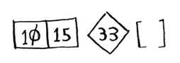

再对子数组进行排序，只包含两个元素的数组（左边的子数组）以及空数组（右边的子数组），快速排序知道如何将他们排序，然后合并结果，就得到一个有序数组。

归纳证明

归纳证明是证明算法行之有效的方式，分为两步：基线条件和归纳条件。
对于快速排序，在基线条件中，证明这种算法对空数组或包含一个元素的数组管用。在归纳条件中，证明快速排序对包含一个元素的数组管用，对包含两个元素的数组也将管用；对两个管用，对三个也管用，以此类推。
下面是快速排序代码：

def quicksort(array):
    if len(array) < 2:
        return array
    else:
        pivot = array[0]
        less = [i for i in array[1:] if i <= pivot]
        greater = [i for i in array[1:] if i > pivot]

        return quicksort(less) + [pivot] + quicksort(greater)

print(quicksort([10, 5, 2, 3]))

第五章 散列表

结合散列函数和数组创建了被称为散列表的数据结构。数组和链表都被直接映射到内存，散列表使用散列函数来确定元素的存储位置。
在Python中，散列表的实现为字典，使用函数dict()来创建。
填装因子：散列表中包含的元素 / 位置总数
散列表可用于数据缓存

第六章 广度优先搜索

队列是一种先进先出的数据结构，而栈是一种后进先出的数据结构。
Pythom中，可以用deque创建一个双端队列

from collections import deque

graph = {"you": ["alice", "bob", "claire"], "bob": ["anuj", "peggy"], "alice": ["peggy"], "claire":["thom", "jonny"], "anuj": [], "peggy": [],
         "thom": [], "jonny": []}


def person_is_seller(name):
    return name[-1] == 'm'


def search(name):
    search_queue = deque()
    search_queue += graph[name]
    searched = []
    while search_queue:
        person = search_queue.popleft()  # 取出第一个人
        if not person in searched:
            if person_is_seller(person):
                print(person + "is a mango seller")
                return True
            else:
                search_queue += graph[person]
                searched.append(person)
    return False

search("you")

注意，若直接搜索图的过程中，因为Peggy既是Alice的朋友又是Bob的朋友因此被加入了两次，搜索队列将包含两个Peggy，所以使用列表进行标记。

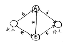
狄克斯特拉算法

狄克斯特拉算法包含的4个步骤：
（1） 找出“最便宜”的节点，即可在最短时间内到达的节点
（2） 更新该节点的邻居的开销
（3） 重复这个过程，直到对图中的每个节点都这样做了
（4） 计算最终路径
这个算法只适用于有向无环图（DAG）。
狄克斯特拉算法不能用于包含负权边的图，在包含负权边的图中找最短路径，可以用另一种算法——贝尔曼-福德算法。
算法实现

graph = {}
graph["you"] = ["alice", "bob", "claire"]
graph["start"] = {}
graph["start"]["a"] = 6
graph["start"]["b"] = 2

graph["a"] = {}
graph["a"]["fin"] = 1

graph["b"] = {}
graph["b"]["a"] = 3
graph["b"]["fin"] = 5

graph["fin"] = {}  # 终点没有邻居

# 接下来 需要散列值存储每个节点的开销
infinity = float("inf")
costs = {}
costs["a"] = 6
costs["b"] = 2
costs["fin"] = infinity

# 还需要一个存储父节点的散列表
parents = {}
parents["a"] = "start"
parents["b"] = "start"
parents["fin"] = None

# 最后需要一个数组，记录处理过的节点
processed = []

def find_lowest_cost_node(costs):
    lowest_cost = float("inf")  # float("inf")表示正无穷
    lowest_cost_node = None
    for node in costs:
        print(node)
        cost = costs[node]
        print(cost)
        if cost < lowest_cost and node not in processed:
            lowest_cost = cost
            lowest_cost_node = node
    return lowest_cost_node


node = find_lowest_cost_node(costs)

while node is not None:
    print(node)
    cost = costs[node]
    print(cost)
    neighbors = graph[node]
    print(neighbors)
    for n in neighbors.keys():
        new_cost = cost + neighbors[n]
        if costs[n] > new_cost:
            costs[n] = new_cost
            parents[n] = node
    processed.append(node)
    node = find_lowest_cost_node(costs)

print(processed)

第八章 贪婪算法