1、简介
孤立森林(Isolation Forest)是另外一种高效的异常检测算法,它和随机森林类似,但每次选择划分属性和划分点(值)时都是随机的,而不是根据信息增益或者基尼指数来选择。在建树过程中,如果一些样本很快就到达了叶子节点(即叶子到根的距离d很短),那么就被认为很有可能是异常点。因为那些路径d比较短的样本,都是因为距离主要的样本点分布中心比较远的。也就是说,可以通过计算样本在所有树中的平均路径长度来寻找异常点。
sklearn提供了ensemble.IsolationForest模块可用于Isolation Forest算法。
2、主要参数和函数介绍
class sklearn.ensemble. IsolationForest ( n_estimators=100 , max_samples=’auto’ , contamination=0.1 , max_features=1.0 , bootstrap=False , n_jobs=1 , random_state=None , verbose=0 )
参数:
n_estimators : int, optional (default=100)
森林中树的颗数
max_samples : int or float, optional (default=”auto”)
对每棵树,样本个数或比例
contamination : float in (0., 0.5), optional (default=0.1)
这是最关键的参数,用户设置样本中异常点的比例
max_features : int or float, optional (default=1.0)
对每棵树,特征个数或比例
函数:
fit(X)
Fit estimator.(无监督)
predict(X)
返回值:+1 表示正常样本, -1表示异常样本。
decision_function(X)
返回样本的异常评分。 值越小表示越有可能是异常样本。
3、IsolationForest实例
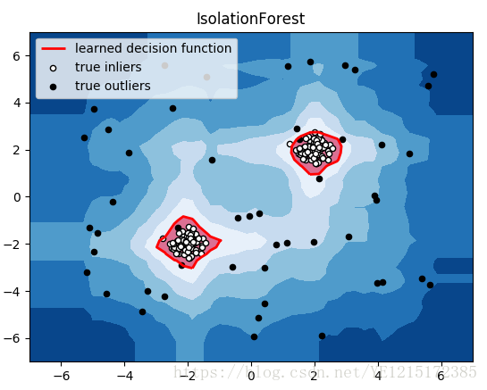
#!/usr/bin/python# -*- coding:utf-8 -*-import numpy as npimport matplotlib.pyplot as pltfrom sklearn.ensemble import IsolationForestfrom scipy import statsrng = np.random.RandomState(42)# 构造训练样本n_samples = 200 #样本总数outliers_fraction = 0.25 #异常样本比例n_inliers = int((1. - outliers_fraction) * n_samples)n_outliers = int(outliers_fraction * n_samples)X = 0.3 * rng.randn(n_inliers // 2, 2)X_train = np.r_[X + 2, X - 2] #正常样本X_train = np.r_[X_train, np.random.uniform(low=-6, high=6, size=(n_outliers, 2))] #正常样本加上异常样本# fit the modelclf = IsolationForest(max_samples=n_samples, random_state=rng, contamination=outliers_fraction)clf.fit(X_train)# y_pred_train = clf.predict(X_train)scores_pred = clf.decision_function(X_train)threshold = stats.scoreatpercentile(scores_pred, 100 * outliers_fraction) #根据训练样本中异常样本比例,得到阈值,用于绘图# plot the line, the samples, and the nearest vectors to the planexx, yy = np.meshgrid(np.linspace(-7, 7, 50), np.linspace(-7, 7, 50))Z = clf.decision_function(np.c_[xx.ravel(), yy.ravel()])Z = Z.reshape(xx.shape)plt.title("IsolationForest")# plt.contourf(xx, yy, Z, cmap=plt.cm.Blues_r)plt.contourf(xx, yy, Z, levels=np.linspace(Z.min(), threshold, 7), cmap=plt.cm.Blues_r) #绘制异常点区域,值从最小的到阈值的那部分a = plt.contour(xx, yy, Z, levels=[threshold], linewidths=2, colors='red') #绘制异常点区域和正常点区域的边界plt.contourf(xx, yy, Z, levels=[threshold, Z.max()], colors='palevioletred') #绘制正常点区域,值从阈值到最大的那部分b = plt.scatter(X_train[:-n_outliers, 0], X_train[:-n_outliers, 1], c='white',s=20, edgecolor='k')c = plt.scatter(X_train[-n_outliers:, 0], X_train[-n_outliers:, 1], c='black',s=20, edgecolor='k')plt.axis('tight')plt.xlim((-7, 7))plt.ylim((-7, 7))plt.legend([a.collections[0], b, c],['learned decision function', 'true inliers', 'true outliers'],loc="upper left")plt.show()
结果:
参考文献:
http://scikit-learn.org/stable/modules/outlier_detection.html#outlier-detection
http://scikit-learn.org/stable/modules/generated/sklearn.ensemble.IsolationForest.html#sklearn.ensemble.IsolationForest