线性回归的从零开始实现

在了解线性回归的关键思想之后，我们可以开始通过代码来动手实现线性回归了。 在这一节中，(我们将从零开始实现整个方法， 包括数据流水线、模型、损失函数和小批量随机梯度下降优化器)。 虽然现代的深度学习框架几乎可以自动化地进行所有这些工作，但从零开始实现可以确保我们真正知道自己在做什么。 同时，了解更细致的工作原理将方便我们自定义模型、自定义层或自定义损失函数。 在这一节中，我们将只使用张量和自动求导。 在之后的章节中，我们会充分利用深度学习框架的优势，介绍更简洁的实现方式。

%matplotlib inline
import random
import torch
from d2l import torch as d2l

%matplotlib inline是一个魔法函数，它能让在Jupyter Notebook中绘制的图表直接在Notebook页面中展示出来。它的作用是在Jupyter Notebook中让图表在运行时显示在页面上，而不是在新窗口中显示。

生成带有噪音的数据集
?=??+?+?.

def synthetic_data(w, b, num_examples):  #@save
    """生成y=Xw+b+噪声"""
    X = torch.normal(0, 1, (num_examples, len(w)))
    y = torch.matmul(X, w) + b
    y += torch.normal(0, 0.01, y.shape)
    return X, y.reshape((-1, 1))

torch.normal(mean,std)       #函数返回从单独的正态分布中提取的随机数的张量，该正态分布的均值是mean，标准差是std。

torch.matmul(x,y)               #矩阵乘法

y.reshape(-1,1)                   # -1 自动计算长度

true_w = torch.tensor([2, -3.4])
true_b = 4.2
features, labels = synthetic_data(true_w, true_b, 1000)

true_w = torch.tensor([2, -3.4])
true_b = 4.2
features, labels = synthetic_data(true_w, true_b, 1000)

d2l.set_figsize()
d2l.plt.scatter(features[:,1], labels, 1);
d2l.plt.show()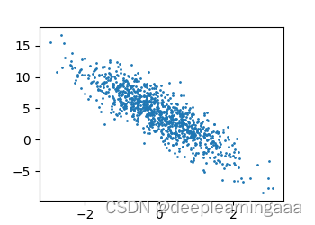

d2l.set_figsize() #表示设置绘制图像的大小，可以进行传参，如果没有进行传参则表示使用默认参数

d2l.plt.scatter() #表示绘制散点图，需要输入两个参数作为横纵坐标。

def data_iter(batch_size, features, labels):
    num_examples = len(features)
    indices = list(range(num_examples))
    # 这些样本是随机读取的，没有特定的顺序
    random.shuffle(indices)
    for i in range(0, num_examples, batch_size):
        batch_indices = torch.tensor(
            indices[i: min(i + batch_size, num_examples)])
        yield features[batch_indices], labels[batch_indices]

 random.shuffle(indices) 将这个列表的排序打乱

yield 在python里面类似于return函数,他们主要的区别就是:遇到return会直接返回值,不会执行接下来的语句.但是yield并不是,在本次迭代返回之后,yield函数在下一次迭代时，从上一次迭代遇到的yield后面的代码(下一行)开始执行