pcd文档快速可视化

一.Linux环境下

1. 安装pcl-tools库

sudo apt-get install pcl-tools

2. 运行pcd文档：

pcl_viewer xxx.pcd

注意：xxx换成对应的pcd文件名

二.win10(linux环境应该也可以），可视化.bin文件

注意 .bin文件时lidar(激光雷达数据常用格式)，上边的.pcd是radar（雷达，应该是超声波雷达，常用数据格式)

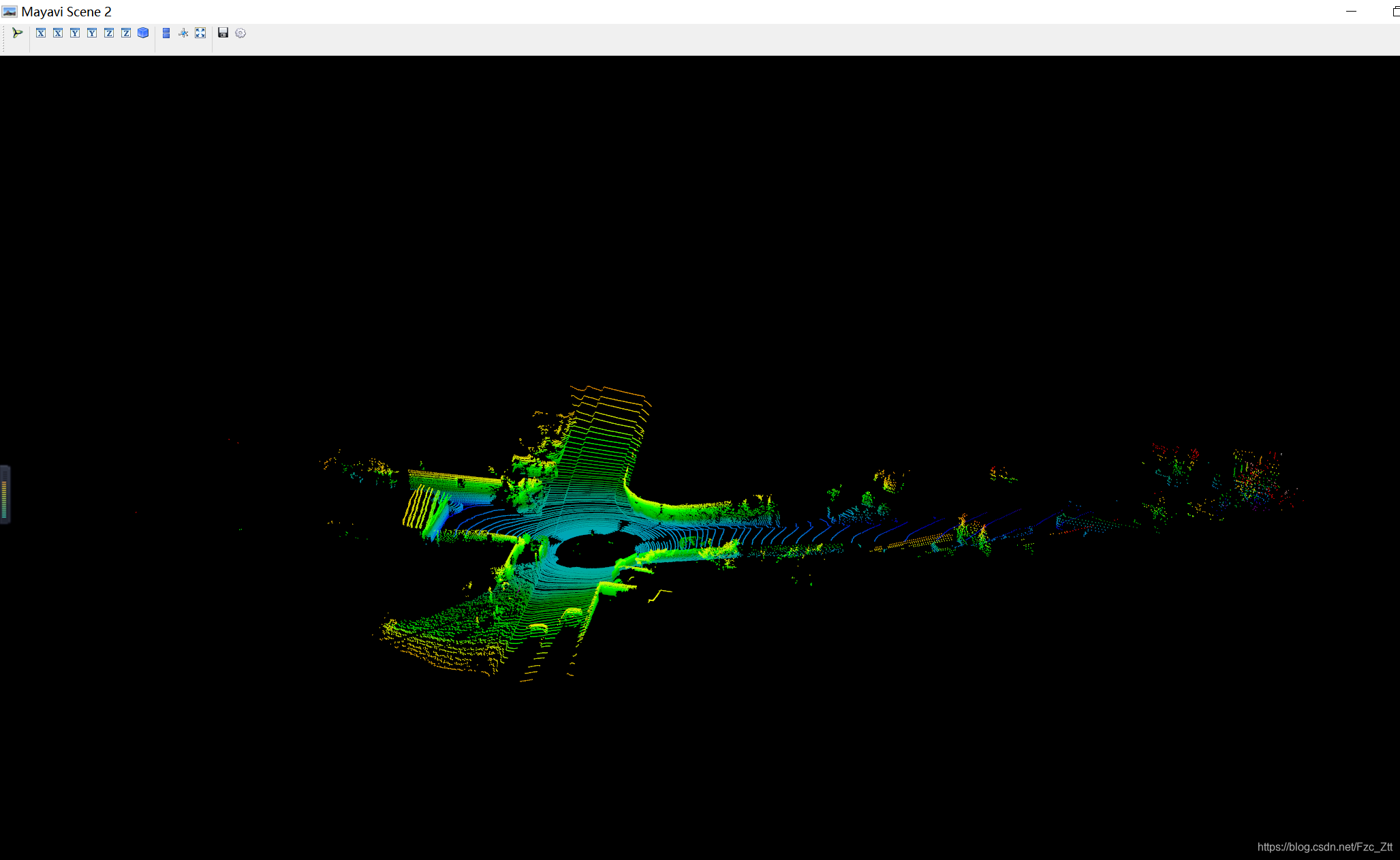
方法一：python中使用numpy读取文件，使用mayavi.mlab包可视化（未安装相应包的先安装包），可视化效果较好，而且可视化界面有一些角度快捷按钮

import numpy as np
import mayavi.mlab
 
# lidar_path换成自己的.bin文件路径
pointcloud2 = np.fromfile(str("H:\\数据集\\KITTI_CSDN\\data_odometry_velodyne\\dataset\\sequences\\11\\velodyne\\000001.bin"), dtype=np.float32, count=-1).reshape([-1, 4])
 
x = pointcloud2[:, 0]  # x position of point
y = pointcloud2[:, 1]  # y position of point
z = pointcloud2[:, 2]  # z position of point
 
r = pointcloud2[:, 3]  # reflectance value of point
d = np.sqrt(x ** 2 + y ** 2)  # Map Distance from sensor
 
degr = np.degrees(np.arctan(z / d))
 
vals = 'height'
if vals == "height":
    col = z
else:
    col = d
 
fig = mayavi.mlab.figure(bgcolor=(0,0,0),size=(640, 500))
mayavi.mlab.points3d(x, y, z,
                     col,  # Values used for Color
                     mode="point",
                     colormap='spectral',  # 'bone', 'copper', 'gnuplot'
                     # color=(0, 1, 0),   # Used a fixed (r,g,b) instead
                     figure=fig,
                     )
 
mayavi.mlab.show()

mayavi效果图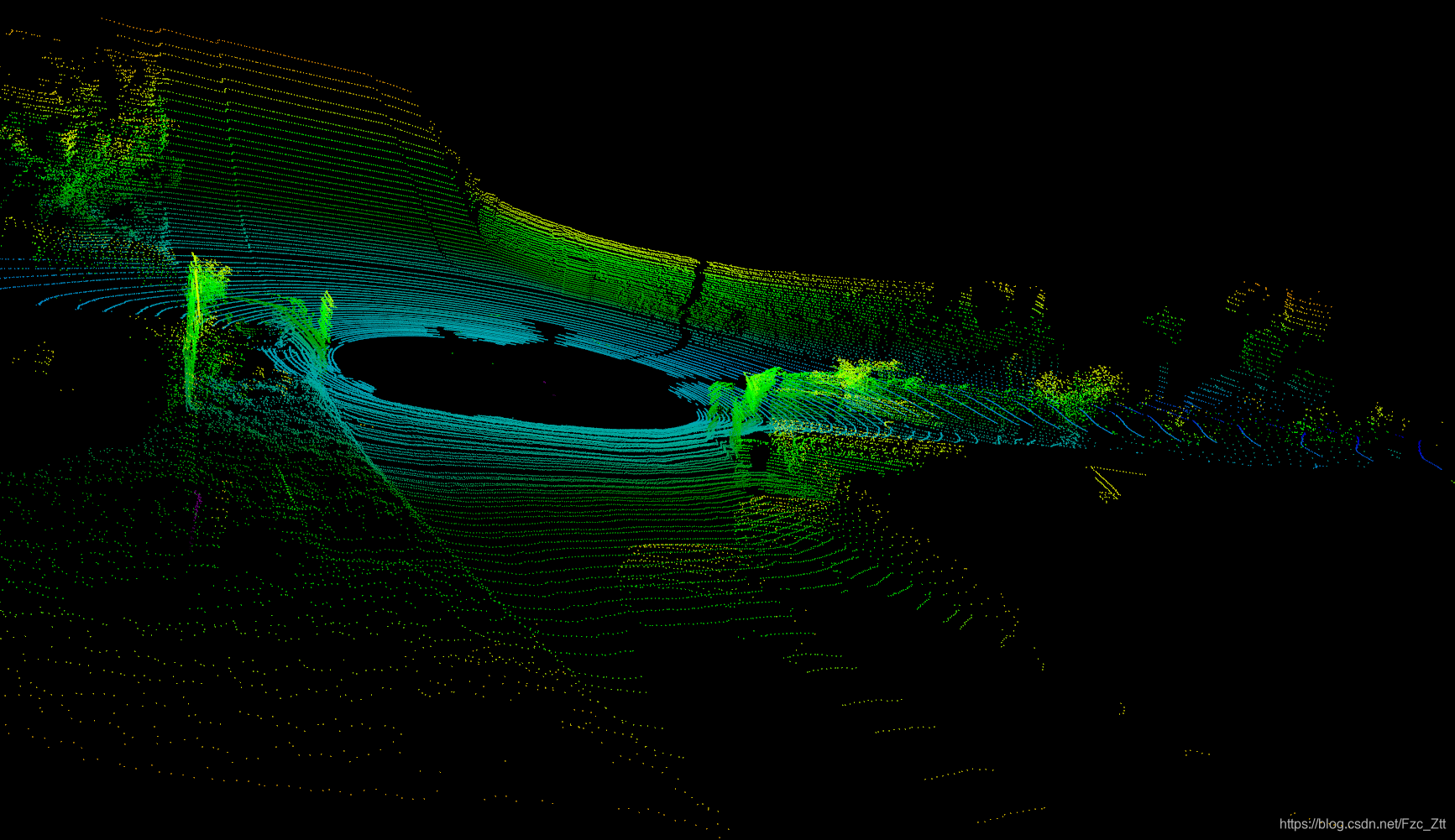

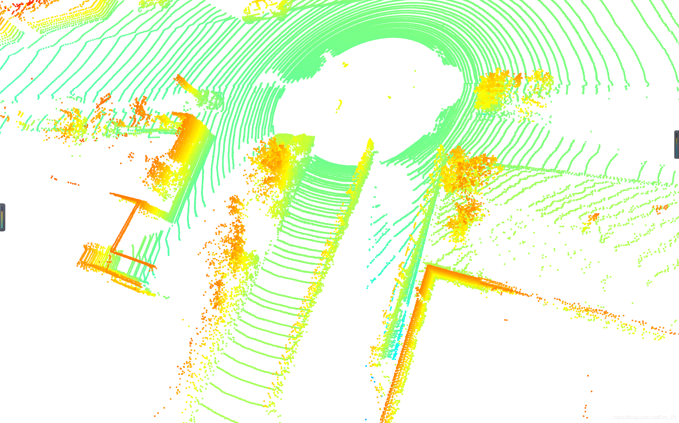
方法二：使用numpy读取，struct包构造，open3d可视化

import os
import numpy as np
import struct
import open3d

def read_bin_velodyne(path):
    pc_list=[]
    with open(path,'rb') as f:
        content=f.read()
        pc_iter=struct.iter_unpack('ffff',content)
        for idx,point in enumerate(pc_iter):
            pc_list.append([point[0],point[1],point[2]])
    return np.asarray(pc_list,dtype=np.float32)

def main():
    root_dir='G:\\kitti_bin\\data_object_velodyne\\testing\\kitti_open3d_test'
    filename=os.listdir(root_dir)
    file_number=len(filename)

    pcd=open3d.open3d.geometry.PointCloud()

    for i in range(file_number):
        path=os.path.join(root_dir, filename[i])
        print(path)
        example=read_bin_velodyne(path)
        # From numpy to Open3D
        pcd.points= open3d.open3d.utility.Vector3dVector(example)
        open3d.open3d.visualization.draw_geometries([pcd])

if __name__=="__main__":
    main()

可视化效果