基于高斯核函数的简单线性回归实现

高斯过程

高斯过程 Gaussian Processes 是概率论和数理统计中随机过程的一种，是多元高斯分布的扩展，被应用于机器学习、信号处理等领域。本文对高斯过程进行公式推导、原理阐述、可视化以及代码实现，介绍了以高斯过程为基础的高斯过程回归 Gaussian Process Regression 基本原理、超参优化、高维输入等问题。

• 一元高斯分布公式
  其概率密度公式如下：
  $$p\left(x\right)=\frac{1}{\sigma \sqrt{2\times \pi }}\exp \left(-\frac{{\left(x-\mu \right)}^2}{2{\sigma }^2}\right)$$

• 核函数(协方差函数)
  核函数是一个高斯过程的核心，核函数决定了一个高斯过程的性质。核函数在高斯过程中起的作用是生成一个协方差矩阵（相关系数矩阵），衡量任意两个点之间的“距离”。最常用的一个核函数为高斯核函数，也成为径向基函数 RBF。其基本形式如下。其中 σ 和 h 是高斯核的超参数。
  $$K\left(x_i,x_j\right)={\sigma }^2\exp \left(-\frac{{\Vert x_i-x_j\Vert }^2}{2h^2}\right)$$
  以下是Python代码实现：

# 定义核函数
   def kernel(self, x1, x2):
       m,n = x1.shape[0], x2.shape[0]
       dist_matrix = np.zeros((m,n), dtype=float)
       for i in range(m):
           for j in range(n):
               dist_matrix[i][j] = np.sum((x1[i]-x2[j])**2)
       return np.exp(-0.5/self.h**2*dist_matrix)

• 作业实现如下：

# 导入相关库
import numpy as np
import matplotlib.pyplot as plt
# 定义高斯过程类
class GPR:
   def __init__(self, h):
       self.is_fit = False
       self.train_x, self.train_y = None, None
       self.h = h
       
   def fit(self, x, y):
       self.train_x = np.asarray(x)
       self.train_y = np.asarray(y)
       self.is_fit = True
       
   def predict(self, x):
       if not self.is_fit:
           print("Sorry! GPR Model can't fit!")
           return
       
       x = np.asarray(x)
       kff = self.kernel(x,x)
       kyy = self.kernel(self.train_x, self.train_x)
       kfy = self.kernel(x, self.train_x)
       kyy_inv =  np.linalg.inv(kyy + 1e-8*np.eye(len(self.train_x)))
       
       mu = kfy.dot(kyy_inv).dot(self.train_y)
       return mu
       
       
   # 定义核函数
   def kernel(self, x1, x2):
       m,n = x1.shape[0], x2.shape[0]
       dist_matrix = np.zeros((m,n), dtype=float)
       for i in range(m):
           for j in range(n):
               dist_matrix[i][j] = np.sum((x1[i]-x2[j])**2)
       return np.exp(-0.5/self.h**2*dist_matrix)

# 创造训练集
train_x = np.arange(0,10).reshape(-1,1)
train_y = np.cos(train_x) + train_x
# 制造槽点
train_y = train_y + np.random.normal(0, 0.01, size=train_x.shape)
# 显示训练集的分布
plt.figure()
plt.scatter(train_x, train_y, label="train", c="red", marker="x")
plt.legend()

输出图：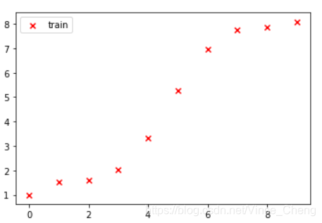

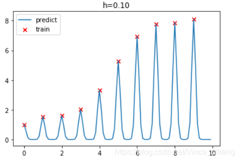
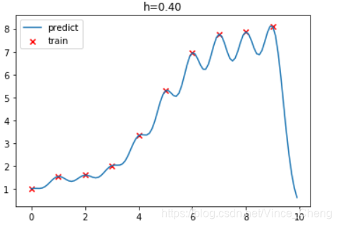
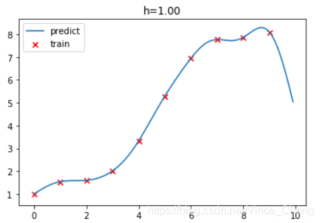
# 创建训练集
test_x = np.arange(0, 10, 0.1).reshape(-1,1)

# 针对不同h值得到拟合图像
h=0.1
for i in range(10):
    gpr = GPR(h)
    gpr.fit(train_x, train_y)
    mu = gpr.predict(test_x)
    test_y = mu.ravel()
    plt.figure()
    plt.title("h=%.2f"%(h))
    plt.plot(test_x, test_y, label="predict")
    plt.scatter(train_x, train_y, label="train", c="red", marker="x")
    plt.legend()
    h += 0.1

输出图像：



参考：
高斯过程
高斯过程浅谈