r roc曲线语言_R语言绘制ROC曲线

librarylibrary(pkgsearch)

找与ROC相关的包

该包会提供一系列关于感兴趣主题的R包，包括他们的评分，作者，连接等等
ps函数等价于pkg_search
size:定义返回结果数量
format="short"返回格式

Sys.setlocale('LC_ALL','C')
rocPkg "ROC",size=200)
head(rocPkg)
class(rocPkg)
[1] "C"
- "ROC" ------------------------------------- 74 packages in 0.01 seconds - 
  #     package     version 
 1  100 pROC        1.15.0  
 2   44 caTools     1.17.1.2
 3   18 survivalROC 1.0.3   
 4   18 PRROC       1.3.1   
 5   15 plotROC     2.2.1   
 6   14 precrec     0.10.1  
 by                                                                       @
 Xavier Robin                                                            2M
 ORPHANED                                                                4M
 Paramita Saha-Chaudhuri000a>  7y
 Jan Grau                                                                1y
 Michael C. Sachs                                                        1y
 Takaya Saito                                                            3M
[1] "pkg_search_result" "tbl_df"            "tbl"              
[4] "data.frame"

ROCR包

performance函数计算tpr,fpr

library(ROCR)
data(ROCR.simple)
df head(df)
##   predictions labels
## 1   0.6125478      1
## 2   0.3642710      1
## 3   0.4321361      0
## 4   0.1402911      0
## 5   0.3848959      0
## 6   0.2444155      1
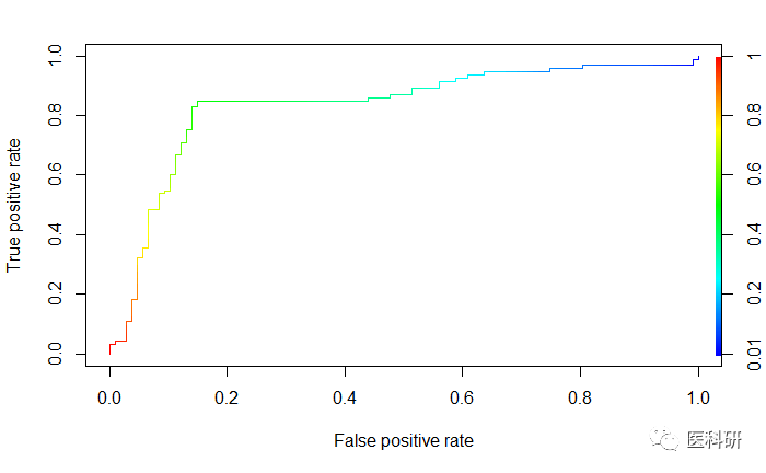
pred perf perf
plot(perf,colorize=TRUE)

plotROC包-ggplot绘制ROC曲线

ROC曲线用于评估连续测量的精度，以预测二进制结果。在医学上，ROC曲线用于评价放射学和一般诊断的诊断试验有着悠久的历史。ROC曲线在信号检测理论中也有很长的应用历史。

require(plotROC)

提供网页版操作，为了代码的连贯性，这里不介绍网页版，不可能我们分析到一般导出数据，拿到网页版去操作。

基本用法

set.seed(2529)
D.ex M1 M2 test                    M1 = M1, M2 = M2, stringsAsFactors = FALSE)
head(test)
##   D   D.str         M1          M2
## 1 1     Ill 1.48117155 -2.50636605
## 2 1     Ill 0.61994478  1.46861033
## 3 0 Healthy 0.57613345  0.07532573
## 4 1     Ill 0.85433197  2.41997703
## 5 0 Healthy 0.05258342  0.01863718
## 6 1     Ill 0.66703989  0.24732453

geom_roc绘图
d为编码1/0, m为用于预测的值marker
注意需要一个disease code,不一定是1/0，但最后选择编码为1/0
如不1/0，则stat_roc默认按顺序最低值为无病状态

basicplot <- ggplot(test, aes(d = D, m = M1)) + geom_roc()basicplot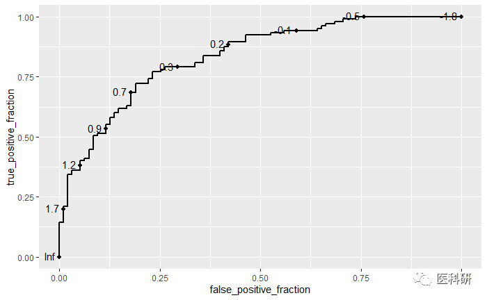

若diseaase编码非1/0:提示warning但仍能继续

ggplot(test, aes(d = D.str, m = M1)) + geom_roc()

n.cuts参数：展示几个截断点
labelsize: 展示标签的大小
labelround: label值保留几位小数

ggplot(test, aes(d = D, m = M1)) + geom_roc(n.cuts = 5, labelsize = 5,  labelround = 2)

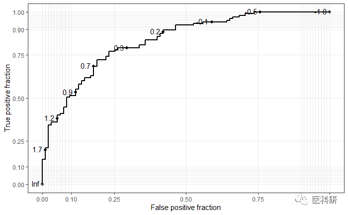
修改style-style_roc函数

styledplot styledplot

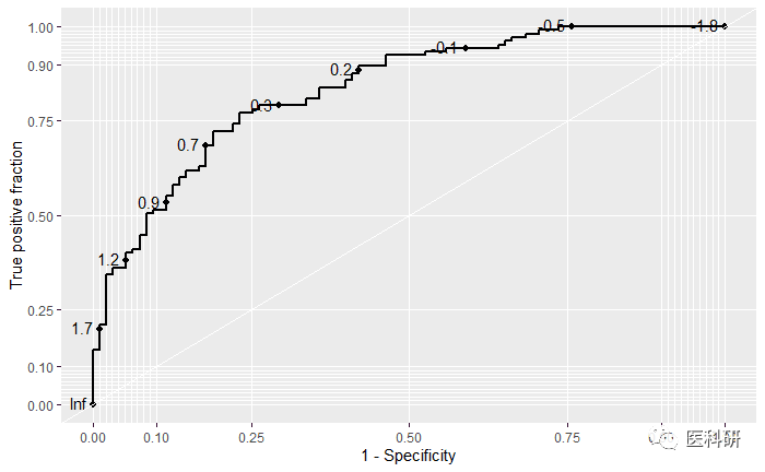
修改xlab, 主题

basicplot + style_roc(theme = theme_grey, xlab = "1 - Specificity")

multiROC-多因素诊断

meltroc类似于dplyr中的gather。转换数据为长数据，原数据为两列marker

head(test)
##     D          M name
## M11 1 1.48117155   M1
## M12 1 0.61994478   M1
## M13 0 0.57613345   M1
## M14 1 0.85433197   M1
## M15 0 0.05258342   M1
## M16 1 0.66703989   M1
longtest head(longtest)
table(longtest$name)

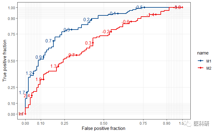
## ROC曲线比较
ggplot(longtest, aes(d = D, m = M, color = name)) + 
  geom_roc() + 
  style_roc()+
  ggsci::scale_color_lancet()

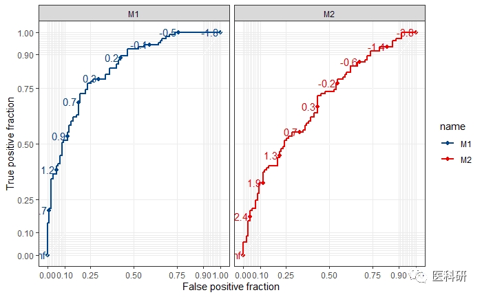
ggplot2分面

ggplot(longtest, aes(d = D, m = M, color = name)) + 
  geom_roc() + 
  style_roc()+
  facet_wrap(~name)+
  ggsci::scale_color_lancet()

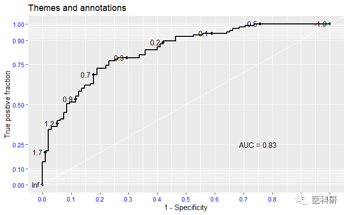
主题与注释
AUC计算并绘制在图中-calc_auc函数
calc_auc(basicplot)$AUC提取

basicplot + 
  style_roc(theme = theme_grey) + ##主题修改
  theme(axis.text = element_text(colour = "blue")) +
  ggtitle("Themes and annotations") + ## 标题
  annotate("text", x = .75, y = .25, ## 注释text的位置
           label = paste("AUC =", round(calc_auc(basicplot)$AUC, 2))) +
  scale_x_continuous("1 - Specificity", breaks = seq(0, 1, by = .1)) ## x刻度
## Scale for 'x' is already present. Adding another scale for 'x', whi

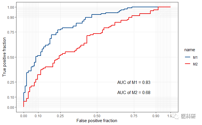
对multi_ROC注释，实现多个AUC值的呈现，实际上仍然是ggplot2语法中的annotate注释

p  geom_roc(n.cuts = 0) + 
  style_roc()+
  ggsci::scale_color_lancet()
auchead(auc)
##   PANEL group      AUC
## 1     1     1 0.833985
## 2     1     2 0.679599
p+annotate("text",x = .75, y = .25, ## 注释text的位置
           label = paste("AUC of M1 =", round(calc_auc(p)$AUC[1], 2))) +
  annotate("text",x = .75, y = .15, ## 注释text的位置)
            label=paste("AUC of M2 =", round(calc_auc(p)$AUC[2], 2)))

其它计算ROC曲线的算法融入

默认的calculate_roc 计算的是 empirical ROC曲线
只要有cutoff, TPF,FPF即可计算，将这些结果以数据框的形式传入到 ggroc 函数
代替默认的统计方法为identity

require(plotROC)
require(ggplot2)
set.seed(2529)
D.ex <- rbinom(200, size = 1, prob = .5)M1 <- rnorm(200, mean = D.ex, sd = .65)M2 <- rnorm(200, mean = D.ex, sd = 1.5)test <- data.frame(D = D.ex, D.str = c("Healthy", "Ill")[D.ex + 1], M1 = M1, M2 = M2, stringsAsFactors = FALSE)head(test)
##   D   D.str         M1          M2
## 1 1     Ill 1.48117155 -2.50636605
## 2 1     Ill 0.61994478  1.46861033
## 3 0 Healthy 0.57613345  0.07532573
## 4 1     Ill 0.85433197  2.41997703
## 5 0 Healthy 0.05258342  0.01863718
## 6 1     Ill 0.66703989  0.24732453D.ex <- test$DM.ex <- test$M1mu1 <- mean(M.ex[D.ex == 1])mu0 <- mean(M.ex[D.ex == 0])s1 <- sd(M.ex[D.ex == 1])s0 <- sd(M.ex[D.ex == 0])c.ex <- seq(min(M.ex), max(M.ex), length.out = 300)
## 构造数据框传入数据binorm.roc <- data.frame(c = c.ex, FPF = pnorm((mu0 - c.ex)/s0), TPF = pnorm((mu1 - c.ex)/s1)
                             )head(binorm.roc)binorm.plot <- ggplot(binorm.roc, aes(x = FPF, y = TPF, label = c)) + geom_roc(stat = "identity") + style_roc(theme = theme_grey)binorm.plot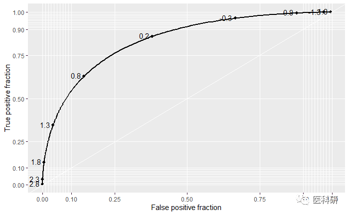

时间依赖的ROC曲线

配合survival ROC包
配合lapply函数实现批量绘图
lappy的结果返回为list，刚好输入do.call

require(ggplot2)
require(plotROC)
library(survivalROC)
survT 350, 1/5)
cens 350, 1, .1)
M -8 * sqrt(survT) + rnorm(350, sd = survT)

### 时间2,5,10
sroc 2, 5, 10), function(t){
  stroc status = cens, marker = M, 
                       predict.time = t, method = "NNE", ## KM法或NNE法
                       span = .25 * 350^(-.2))
  data.frame(TPF = stroc[["TP"]], FPF = stroc[["FP"]], 
             c = stroc[["cut.values"]], 
             time = rep(stroc[["predict.time"]], length(stroc[["FP"]])))
})

## 整合到数据框中
sroclong do.call(rbind, sroc)
class(sroclong)
## [1] "data.frame"
head(sroclong)
##   TPF       FPF         c time
## 1   1 1.0000000      -Inf    2
## 2   1 0.9970286 -96.21091    2
## 3   1 0.9940573 -89.13315    2
## 4   1 0.9910859 -80.53402    2
## 5   1 0.9881145 -70.53104    2
## 6   1 0.9851431 -67.81392    2
sroclong$timetime)

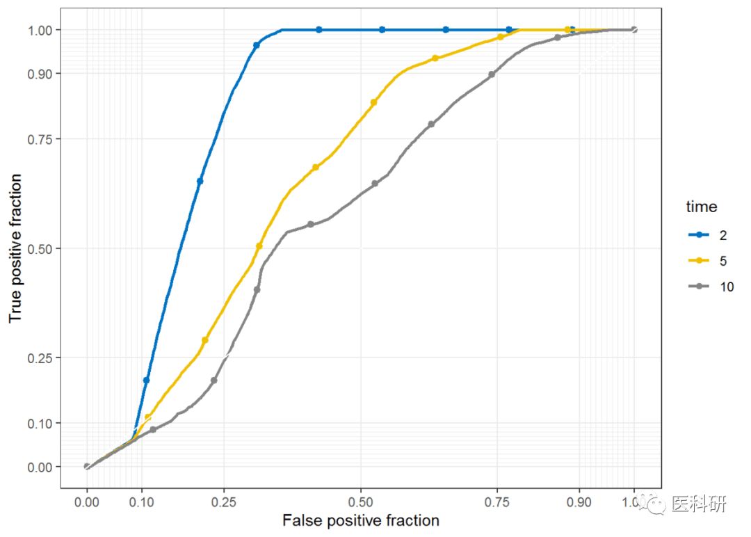
## 绘制ROC
pROCtime)) + 
  geom_roc(labels = FALSE, stat = "identity") + 
  style_roc()+
  ggsci::scale_color_jco()
pROC

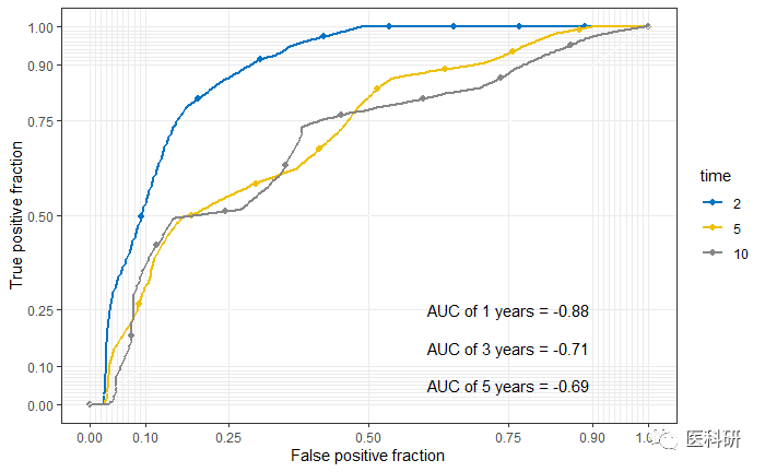
添加注释

pROC+annotate("text",x = .75, y = .25, ## 注释text的位置
           label = paste("AUC of 1 years =", round(calc_auc(pROC)$AUC[1], 2))) +
     annotate("text",x = .75, y = .15, ## 注释text的位置)
            label=paste("AUC of 3 years =", round(calc_auc(pROC)$AUC[2], 2)))+
     annotate("text",x = .75, y = .05, ## 注释text的位置)
            label=paste("AUC of 5 years =", round(calc_auc(pROC)$AUC[3], 2)))

原文链接：https://blog.csdn.net/weixin_39622901/article/details/111645786