自从搞了简单的文字识别之后,就在考虑机器视觉还能为我的研究生盆子上镶点什么金边,简单搜了一下文献,对于刀具磨损的视觉识别还是不少的,但是要么是拆下来拍照检测,要么是固定在某个位置检测,机器视觉还没有真正实现在机检测,又去某国内学术网站搜了一下,发现这个东西够一篇硕士毕业论文了,那还是简单搞搞吧。
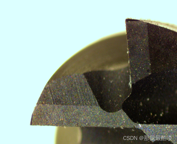
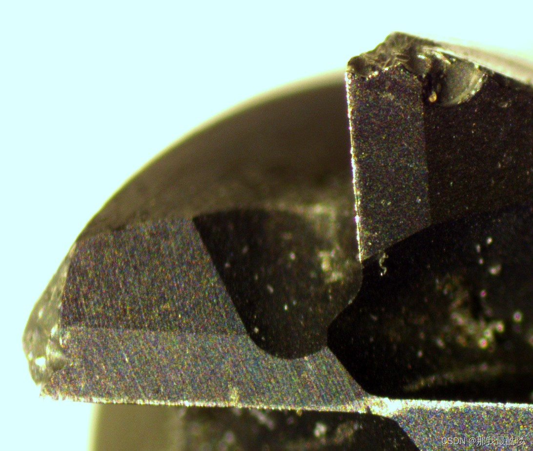
wear tool应该与new tool进行轮廓对比,所以就需要得到两种刀具的轮廓。下面是我的new tool和wear tool:
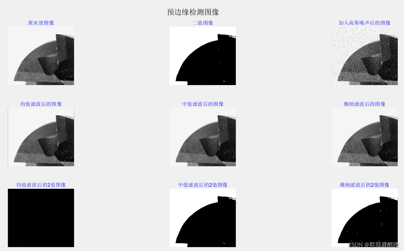
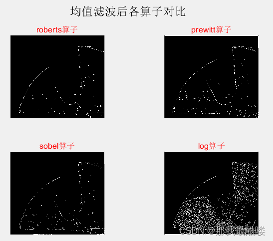
边缘检测就是算法,直接上代码了。我对各个滤波方法和边缘检测算子进行了对比,代码和对比结果如下:
%比较滤波效果
A = imread('D:\Users\weixi\MATLAB\Projects\cv_edge\new.jpg');%读入彩色图片
B=rgb2gray(A);%把彩色图片转化成灰度图片,256级
B_gaosi=imnoise(B,'gaussian');%加入高斯噪声
h=fspecial('average',6);%fspecial函数用于预定义滤波器
A_junzhi=uint8(round(filter2(h,B)));%进行均值滤波
A_zhongzhi=medfilt2(B,[8,8]);%进行中值滤波
A_weina=wiener2(B,[8,8]);%进行维纳滤波
i_max=double(max(max(B))); %获取亮度最大值
i_min=double(min(min(B))); %获取亮度最小值
thresh=round(i_max-((i_max-i_min)/3)); %计算灰度图像转化成二值图像的门限thresh
B_2=(B>=thresh); %B_2为二值图像
A_junzhi_2=uint8(round(filter2(h,B_2)));%进行均值滤波
A_zhongzhi_2=medfilt2(B_2,[3,3]);%进行中值滤波
A_weina_2=wiener2(B_2,[3,3]);%进行维纳滤波
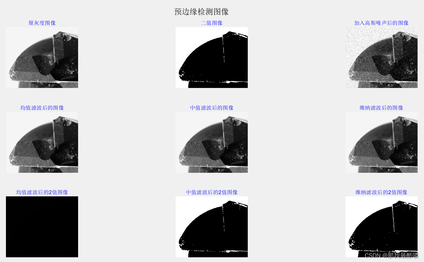
figure(1);
subplot(3,3,1);imshow(B);title('原灰度图像','color','b');
subplot(3,3,2);imshow(B_2);title('二值图像','color','b');
subplot(3,3,3);imshow(B_gaosi);title('加入高斯噪声后的图像','color','b');
subplot(3,3,4);imshow(A_junzhi);title('均值滤波后的图像','color','b');
subplot(3,3,5);imshow(A_zhongzhi);title('中值滤波后的图像','color','b');
subplot(3,3,6);imshow(A_weina);title('维纳滤波后的图像','color','b');
subplot(3,3,7);imshow(A_junzhi_2);title('均值滤波后的2值图像','color','b');
subplot(3,3,8);imshow(A_zhongzhi_2);title('中值滤波后的2值图像','color','b');
subplot(3,3,9);imshow(A_weina_2);title('维纳滤波后的2值图像','color','b');
sgtitle('预边缘检测图像');
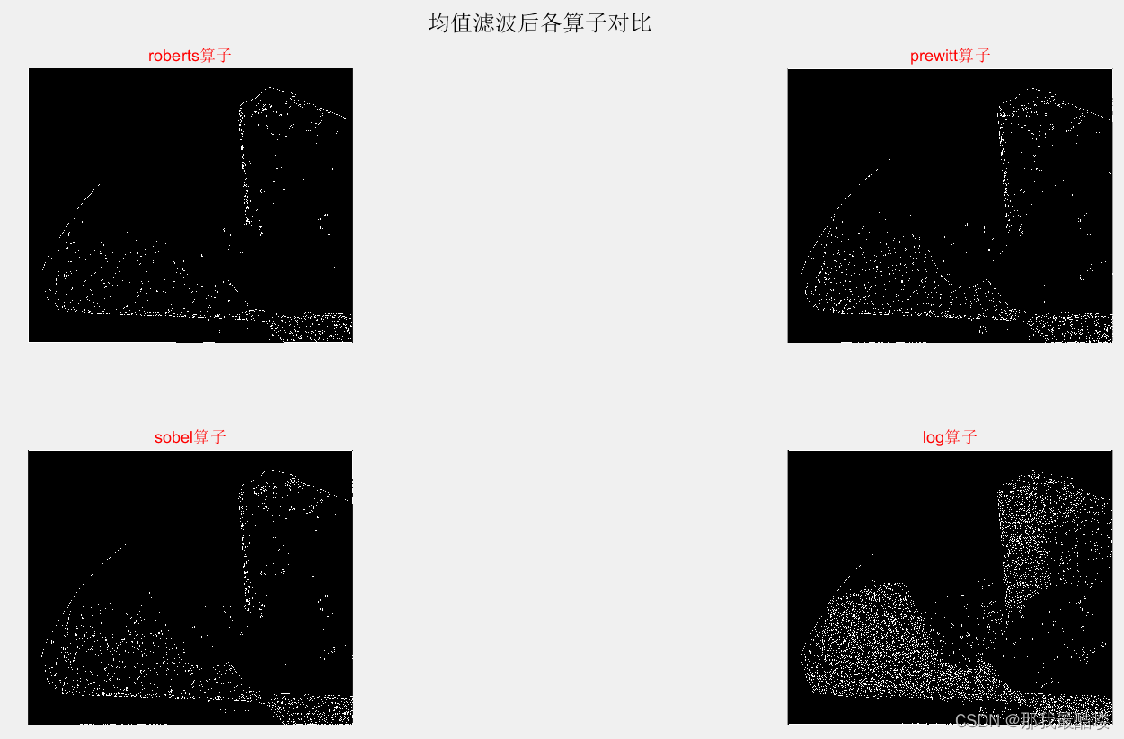
figure(2);
AW1=edge(A_junzhi,'roberts');AW1_2=edge(A_junzhi_2,'roberts');
AW2=edge(A_junzhi,'prewitt');AW2_2=edge(A_junzhi_2,'prewitt');
AW3=edge(A_junzhi,'sobel');AW3_2=edge(A_junzhi_2,'sobel');
AW4=edge(A_junzhi,'log');AW4_2=edge(A_junzhi_2,'log');
subplot(2,2,1),imshow(AW1),title('roberts算子','color','r');
subplot(2,2,2),imshow(AW2),title('prewitt算子','color','r');
subplot(2,2,3),imshow(AW3),title('sobel算子','color','r');
subplot(2,2,4),imshow(AW4),title('log算子','color','r');
sgtitle('均值滤波后各算子对比');
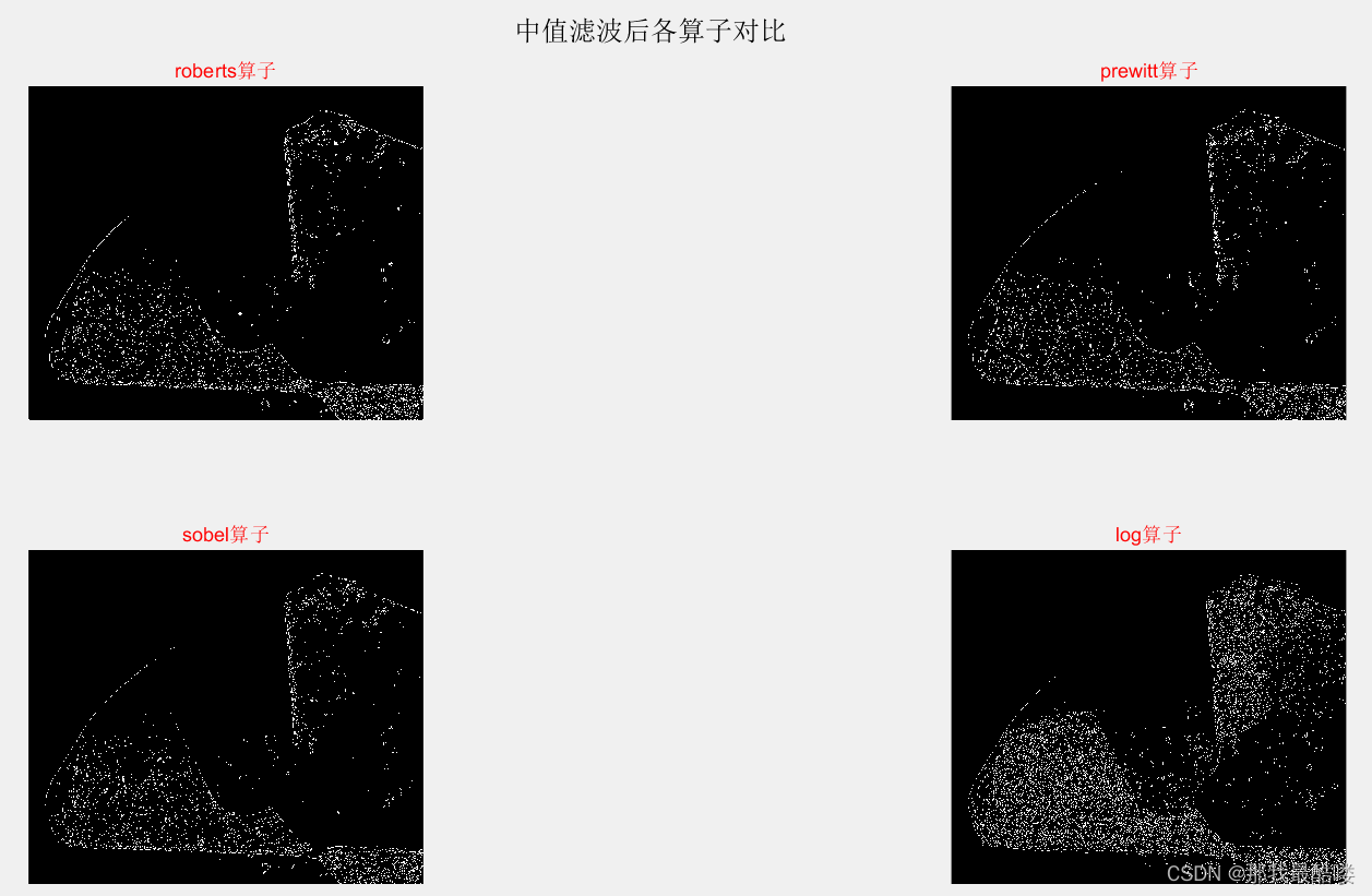
figure(3);
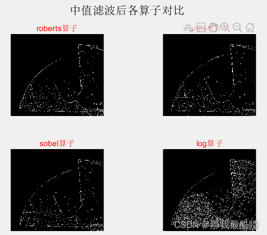
BW1=edge(A_zhongzhi,'roberts');
BW2=edge(A_zhongzhi,'prewitt');
BW3=edge(A_zhongzhi,'sobel');
BW4=edge(A_zhongzhi,'log');
BW1_2=edge(A_zhongzhi_2,'roberts');
BW2_2=edge(A_zhongzhi_2,'prewitt');
BW3_2=edge(A_zhongzhi_2,'sobel');
BW4_2=edge(A_zhongzhi_2,'log');
subplot(2,2,1),imshow(BW1),title('roberts算子','color','r');
subplot(2,2,2),imshow(BW2),title('prewitt算子','color','r');
subplot(2,2,3),imshow(BW3),title('sobel算子','color','r');
subplot(2,2,4),imshow(BW4),title('log算子','color','r');
sgtitle('中值滤波后各算子对比');
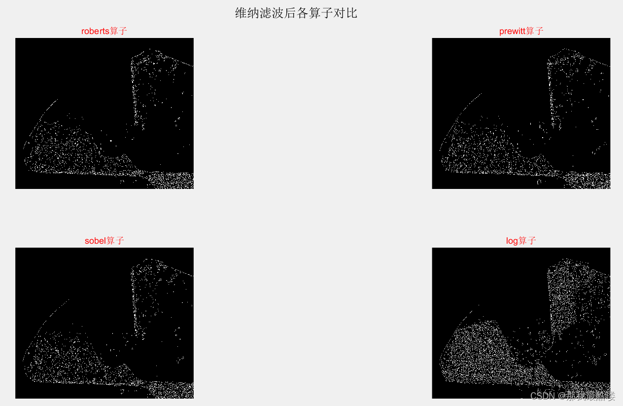
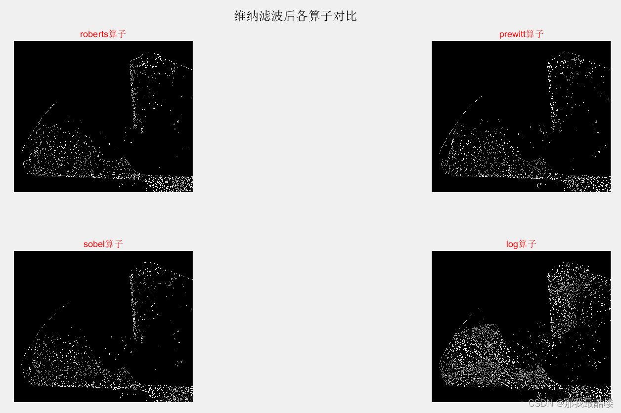
figure(4);
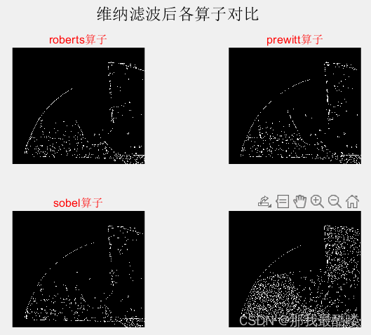
CW1=edge(A_weina,'roberts');
CW2=edge(A_weina,'prewitt');
CW3=edge(A_weina,'sobel');
CW4=edge(A_weina,'log');
CW1_2=edge(A_weina_2,'roberts');
CW2_2=edge(A_weina_2,'prewitt');
CW3_2=edge(A_weina_2,'sobel');
CW4_2=edge(A_weina_2,'log');
subplot(2,2,1),imshow(CW1),title('roberts算子','color','r');
subplot(2,2,2),imshow(CW2),title('prewitt算子','color','r');
subplot(2,2,3),imshow(CW3),title('sobel算子','color','r');
subplot(2,2,4),imshow(CW4),title('log算子','color','r');
sgtitle('维纳滤波后各算子对比');
figure(5);
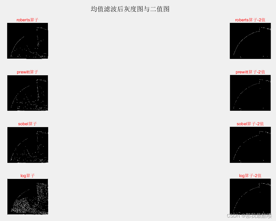
subplot(4,2,1),imshow(AW1),title('roberts算子','color','r');
subplot(4,2,2),imshow(AW1_2),title('roberts算子-2值','color','r');
subplot(4,2,3),imshow(AW2),title('prewitt算子','color','r');
subplot(4,2,4),imshow(AW2_2),title('prewitt算子-2值','color','r');
subplot(4,2,5),imshow(AW3),title('sobel算子','color','r');
subplot(4,2,6),imshow(AW3_2),title('sobel算子-2值','color','r');
subplot(4,2,7),imshow(AW4),title('log算子','color','r');
subplot(4,2,8),imshow(AW4_2),title('log算子-2值','color','r');
sgtitle('均值滤波后灰度图与二值图');
figure(6);
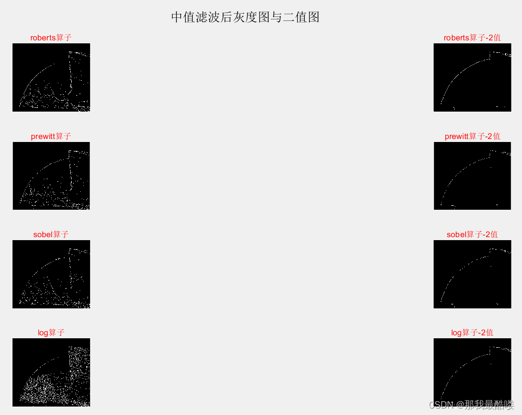
subplot(4,2,1),imshow(BW1),title('roberts算子','color','r');
subplot(4,2,2),imshow(BW1_2),title('roberts算子-2值','color','r');
subplot(4,2,3),imshow(BW2),title('prewitt算子','color','r');
subplot(4,2,4),imshow(BW2_2),title('prewitt算子-2值','color','r');
subplot(4,2,5),imshow(BW3),title('sobel算子','color','r');
subplot(4,2,6),imshow(BW3_2),title('sobel算子-2值','color','r');
subplot(4,2,7),imshow(BW4),title('log算子','color','r');
subplot(4,2,8),imshow(BW4_2),title('log算子-2值','color','r');
sgtitle('中值滤波后灰度图与二值图');
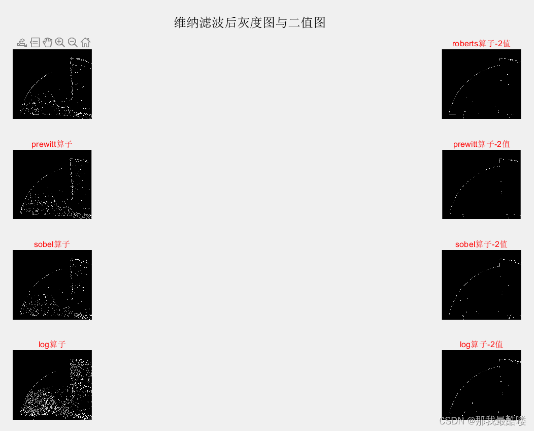
figure(7);
subplot(4,2,1),imshow(CW1),title('roberts算子','color','r');
subplot(4,2,2),imshow(CW1_2),title('roberts算子-2值','color','r');
subplot(4,2,3),imshow(CW2),title('prewitt算子','color','r');
subplot(4,2,4),imshow(CW2_2),title('prewitt算子-2值','color','r');
subplot(4,2,5),imshow(CW3),title('sobel算子','color','r');
subplot(4,2,6),imshow(CW3_2),title('sobel算子-2值','color','r');
subplot(4,2,7),imshow(CW4),title('log算子','color','r');
subplot(4,2,8),imshow(CW4_2),title('log算子-2值','color','r');
sgtitle('维纳滤波后灰度图与二值图');new tool
wear tool
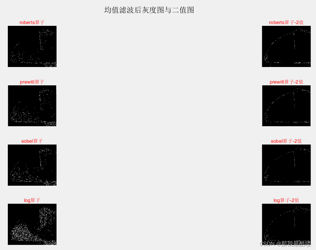
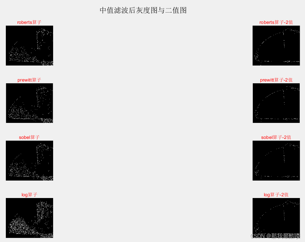
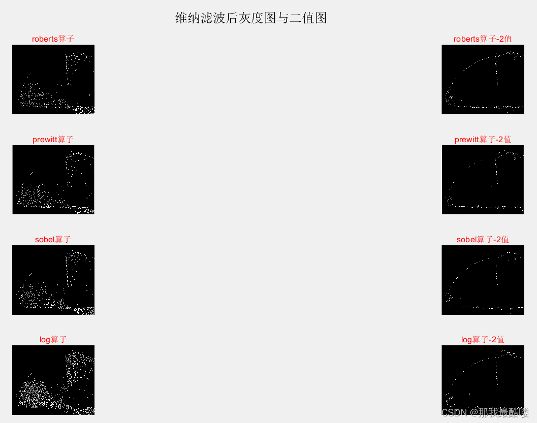
可以看出由二值图像得出的轮廓边缘比较清晰,由灰度图得到一些模糊的其他磨损特征
后续再研究吧。
ps:matlab牛bi~(破音)
版权声明:本文为Breathmetoyou原创文章,遵循CC 4.0 BY-SA版权协议,转载请附上原文出处链接和本声明。