最小二乘法和正则化

高斯于1823年在误差e1 ,… , en独立同分布的假定下,证明了最小二乘方法的一个最优性质: 在所有无偏的线性估计类中,最小二乘方法是其中方差最小的！

使用最小二乘法拟和曲线

对于数据$(x_i,y_i)(i=1,2,3...,m)$

拟合出函数$h(x)$

有误差，即残差：$r_i=h(x_i)-y_i$

此时L2范数(残差平方和)最小时，h(x) 和 y 相似度最高，更拟合

一般的H(x)为n次的多项式，$H(x)=w_0+w_{1}x+w_2{x}^2+...w_n{x}^n$

$w(w_0,w_1,w_2,...,w_n)$为参数

最小二乘法就是要找到一组 $w(w_0,w_1,w_2,...,w_n)$ 使得${\sum }_{i=1}^n(h(x_i)-y_i{)}^2$ (残差平方和) 最小

即，求 $min{\sum }_{i=1}^n(h(x_i)-y_i{)}^2$

举例：我们用目标函数$y=sin2\pi x$, 加上一个正太分布的噪音干扰，用多项式去拟合【例1.1 11页】

import numpy as np
import scipy as sp
from scipy.optimize import leastsq
import matplotlib.pyplot as plt
%matplotlib inline

ps: numpy.poly1d([1,2,3]) 生成 $1x^2+2x^1+3x^0$

# 目标函数
def real_func(x):
    return np.sin(2*np.pi*x)

# 多项式
def fit_func(p, x):
    f = np.poly1d(p)
    return f(x)

# 残差
def residuals_func(p, x, y): #p应该是初始参数，是多项式前面的系数a，b，c等
    ret = fit_func(p, x) - y
    return ret

# 十个点
x = np.linspace(0, 1, 10)
x_points = np.linspace(0, 1, 1000)
# 加上正态分布噪音的目标函数的值
y_ = real_func(x)
y = [np.random.normal(0, 0.1)+y1 for y1 in y_]

def fitting(M=0):
    """
    M    为 多项式的次数
    """    
    # 随机初始化多项式参数
    p_init = np.random.rand(M+1)
    # 最小二乘法
    p_lsq = leastsq(residuals_func, p_init, args=(x, y))
    print('Fitting Parameters:', p_lsq[0])
    
    # 可视化
    plt.plot(x_points, real_func(x_points), label='real')
    plt.plot(x_points, fit_func(p_lsq[0], x_points), label='fitted curve')
    plt.plot(x, y, 'bo', label='noise')
    plt.legend()
    return p_lsq

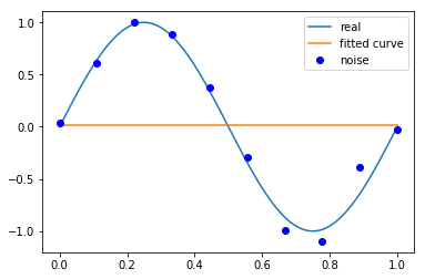
# M=0
p_lsq_0 = fitting(M=0)

Fitting Parameters: [0.01191424]

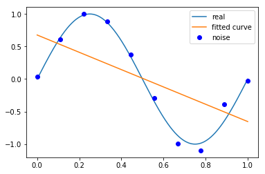
# M=1
p_lsq_1 = fitting(M=1)

Fitting Parameters: [-1.33036473  0.6770966 ]

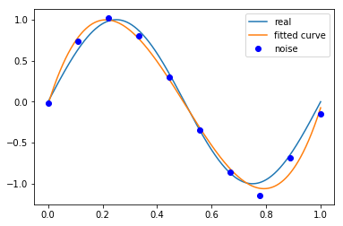
# M=3
p_lsq_3 = fitting(M=3)

Fitting Parameters: [ 21.14354912 -31.85091     10.66661731  -0.03324716]

# M=9
p_lsq_9 = fitting(M=9)

Fitting Parameters: [ 7.45555674e+03 -3.31796363e+04  6.14569910e+04 -6.14712518e+04
  3.59846685e+04 -1.24263822e+04  2.40975039e+03 -2.44841906e+02
  1.50820818e+01  4.16353905e-02]

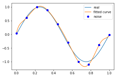
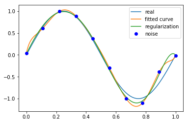
当M=9时，多项式曲线通过了每个数据点，但是造成了过拟合

正则化

结果显示过拟合， 引入正则化项(regularizer)，降低过拟合

$Q(x)={\sum }_{i=1}^n(h(x_i)-y_i{)}^2+\lambda ||w|{|}^2$。

回归问题中，损失函数是平方损失，正则化可以是参数向量的L2范数,也可以是L1范数。

• L1: regularization*abs§

• L2: 0.5 * regularization * np.square§

regularization = 0.0001

def residuals_func_regularization(p, x, y):
    ret = residuals_func(p, x, y)
    ret = np.append(ret, np.sqrt(0.5*regularization*np.square(p))) # L2范数作为正则化项
    return ret

# 最小二乘法,加正则化项
p_init = np.random.rand(9+1)
p_lsq_regularization = leastsq(residuals_func_regularization, p_init, args=(x, y))

plt.plot(x_points, real_func(x_points), label='real')
plt.plot(x_points, fit_func(p_lsq_9[0], x_points), label='fitted curve')
plt.plot(x_points, fit_func(p_lsq_regularization[0], x_points), label='regularization')
plt.plot(x, y, 'bo', label='noise')
plt.legend()

<matplotlib.legend.Legend at 0x22e88ece9b0>

原文代码作者：https://github.com/wzyonggege/statistical-learning-method

中文注释制作：机器学习初学者