CV方向

1.图像增广

1.1.概念

1.1.1.大规模数据集是成功应用深度神经网络的前提
1.1.2.图像增广（image augmentation）技术通过对训练图像做一系列随机改变，来产生相似但又不同的训练样本，从而扩大训练数据集的规模
1.1.3.另一种解释是，随机改变训练样本可以降低模型对某些属性的依赖，从而提高模型的泛化能力。

1.2.准备工作

1.2.1.首先，导入实验所需的包或模块

%matplotlib inline
import os
import time
import torch
from torch import nn, optim
from torch.utils.data import Dataset, DataLoader
import torchvision
import sys
from PIL import Image

sys.path.append("/home/kesci/input/")
#置当前使用的GPU设备仅为0号设备
os.environ["CUDA_VISIBLE_DEVICES"] = "0"   

import d2lzh1981 as d2l

# 定义device，是否使用GPU，依据计算机配置自动会选择
device = torch.device('cuda' if torch.cuda.is_available() else 'cpu')
print(torch.__version__)
print(device)

1.2.2.读取一张图像作为实验的样例

d2l.set_figsize()
img = Image.open('/home/kesci/input/img2083/img/cat1.jpg')
d2l.plt.imshow(img)

1.2.3.定义绘图函数show_images

# 本函数已保存在d2lzh_pytorch包中方便以后使用
def show_images(imgs, num_rows, num_cols, scale=2):
    figsize = (num_cols * scale, num_rows * scale)
    _, axes = d2l.plt.subplots(num_rows, num_cols, figsize=figsize)
    for i in range(num_rows):
        for j in range(num_cols):
            axes[i][j].imshow(imgs[i * num_cols + j])
            axes[i][j].axes.get_xaxis().set_visible(False)
            axes[i][j].axes.get_yaxis().set_visible(False)
    return axes

1.2.4.定义一个辅助函数apply
这个函数对输入图像img多次运行图像增广方法aug并展示所有的结果

def apply(img, aug, num_rows=2, num_cols=4, scale=1.5):
    Y = [aug(img) for _ in range(num_rows * num_cols)]
    show_images(Y, num_rows, num_cols, scale)

1.3.常用的图像增广方法

1.3.1.翻转和裁剪
左右翻转图像通常不改变物体的类别，它是最早也是最广泛使用的一种图像增广方法
• 我们通过torchvision.transforms模块创建RandomHorizontalFlip实例来实现一半概率的图像水平（左右）翻转

apply(img, torchvision.transforms.RandomHorizontalFlip())

上下翻转不如左右翻转通用
• 创建RandomVerticalFlip实例来实现一半概率的图像垂直（上下）翻转。

apply(img, torchvision.transforms.RandomVerticalFlip())

通过对图像随机裁剪来让物体以不同的比例出现在图像的不同位置，这同样能够降低模型对目标位置的敏感性。
• 每次随机裁剪出一块面积为原面积10%~100%的区域，且该区域的宽和高之比随机取自0.5-2，然后再将该区域的宽和高分别缩放到200像素。若无特殊说明，本节中a和b之间的随机数指的是从区间[a,b]中随机均匀采样所得到的连续值。

shape_aug = torchvision.transforms.RandomResizedCrop(200, scale=(0.1, 1), ratio=(0.5, 2))
apply(img, shape_aug)

1.3.2.变化颜色
亮度（参数brightness）

apply(img, torchvision.transforms.ColorJitter(brightness=0.5, contrast=0, saturation=0, hue=0))

对比度（参数contrast）

apply(img, torchvision.transforms.ColorJitter(brightness=0, contrast=0.5, saturation=0, hue=0))

饱和度（参数saturation）
色调（参数hue）

apply(img, torchvision.transforms.ColorJitter(brightness=0, contrast=0, saturation=0, hue=0.5))

可以同时变换多个参数

color_aug = torchvision.transforms.ColorJitter(brightness=0.5, contrast=0.5, saturation=0.5, hue=0.5)
apply(img, color_aug)

1.3.3.叠加多个图像增广方法
实际应用中我们会将多个图像增广方法叠加使用。我们可以通过Compose实例将上面定义的多个图像增广方法叠加起来，再应用到每张图像之上。

ugs = torchvision.transforms.Compose([
    torchvision.transforms.RandomHorizontalFlip(), color_aug, shape_aug])
apply(img, augs)

1.4.使用图像增广训练模型

1.4.1.使用CIFAR-10数据集

CIFAR_ROOT_PATH = '/home/kesci/input/cifar102021'
all_imges = torchvision.datasets.CIFAR10(train=True, root=CIFAR_ROOT_PATH, download = True)
# all_imges的每一个元素都是(image, label)
show_images([all_imges[i][0] for i in range(32)], 4, 8, scale=0.8);

1.4.2.为了在预测时得到确定的结果，我们通常只将图像增广应用在训练样本上，而不在预测时使用含随机操作的图像增广。使用ToTensor将小批量图像转成PyTorch需要的格式，即形状为(批量大小, 通道数, 高, 宽)、值域在0到1之间且类型为32位浮点数。

flip_aug = torchvision.transforms.Compose([
     torchvision.transforms.RandomHorizontalFlip(),
     torchvision.transforms.ToTensor()])

no_aug = torchvision.transforms.Compose([
     torchvision.transforms.ToTensor()])

1.4.3.定义一个辅助函数来方便读取图像并应用图像增广

num_workers = 0 if sys.platform.startswith('win32') else 4
def load_cifar10(is_train, augs, batch_size, root=CIFAR_ROOT_PATH):
    dataset = torchvision.datasets.CIFAR10(root=root, train=is_train, transform=augs, download=False)
    return DataLoader(dataset, batch_size=batch_size, shuffle=is_train, num_workers=num_workers)

1.4.4.定义train函数：使用GPU训练并评价模型（ResNet-18模型）

# 本函数已保存在d2lzh_pytorch包中方便以后使用
def train(train_iter, test_iter, net, loss, optimizer, device, num_epochs):
    net = net.to(device)
    print("training on ", device)
    batch_count = 0
    for epoch in range(num_epochs):
        train_l_sum, train_acc_sum, n, start = 0.0, 0.0, 0, time.time()
        for X, y in train_iter:
            X = X.to(device)
            y = y.to(device)
            y_hat = net(X)
            l = loss(y_hat, y)
            optimizer.zero_grad()
            l.backward()
            optimizer.step()
            train_l_sum += l.cpu().item()
            train_acc_sum += (y_hat.argmax(dim=1) == y).sum().cpu().item()
            n += y.shape[0]
            batch_count += 1
        test_acc = d2l.evaluate_accuracy(test_iter, net)
        print('epoch %d, loss %.4f, train acc %.3f, test acc %.3f, time %.1f sec'
              % (epoch + 1, train_l_sum / batch_count, train_acc_sum / n, test_acc, time.time() - start))

1.4.5.定义train_with_data_aug函数使用图像增广来训练模型，使用Adam算法作为训练使用的优化算法，然后将图像增广应用于训练数据集之上，最后调用刚才定义的train函数训练并评价模型。

def train_with_data_aug(train_augs, test_augs, lr=0.001):
    batch_size, net = 256, d2l.resnet18(10)
    optimizer = torch.optim.Adam(net.parameters(), lr=lr)
    loss = torch.nn.CrossEntropyLoss()
    train_iter = load_cifar10(True, train_augs, batch_size)
    test_iter = load_cifar10(False, test_augs, batch_size)
    train(train_iter, test_iter, net, loss, optimizer, device, num_epochs=10)

# 使用随机左右翻转的图像增广来训练模型
train_with_data_aug(flip_aug, no_aug)

2.模型微调

2.1.概念

2.1.1.迁移学习中的一种常用技术：微调（fine tuning），微调由以下4步构成

在源数据集（大型数据集，如ImageNet数据集）上预训练一个神经网络模型，即源模型。
创建一个新的神经网络模型，即目标模型（一般数据集不是很大）。它复制了源模型上“除了输出层外”的所有模型设计及其参数。我们假设这些模型参数包含了源数据集上学习到的知识，且这些知识同样适用于目标数据集。我们还假设源模型的输出层跟源数据集的标签紧密相关，因此在目标模型中不予采用。
为目标模型添加一个输出大小为目标数据集类别个数的输出层，并随机初始化该层的模型参数。
在目标数据集（如椅子数据集）上训练目标模型。我们将从头训练输出层，而其余层的参数都是基于源模型的参数微调得到的。
2.1.2.当目标数据集远小于源数据集时，微调有助于提升模型的泛化能力。

2.2.实例：热狗识别

2.2.1.首先，导入实验所需的包或模块
torchvision的models包提供了常用的预训练模型
若想获取更多的预训练模型，可以使用使用pretrained-models.pytorch仓库。

%matplotlib inline
import torch
from torch import nn, optim
from torch.utils.data import Dataset, DataLoader
import torchvision
from torchvision.datasets import ImageFolder
from torchvision import transforms
from torchvision import models
import os

import sys

sys.path.append("/home/kesci/input/")
import d2lzh1981 as d2l

os.environ["CUDA_VISIBLE_DEVICES"] = "0"
device = torch.device('cuda' if torch.cuda.is_available() else 'cpu')

2.2.2.获取数据集

import os
os.listdir('/home/kesci/input/resnet185352')

data_dir = '/home/kesci/input/hotdog4014'
os.listdir(os.path.join(data_dir, "hotdog"))

我们创建两个ImageFolder实例来分别读取训练数据集和测试数据集中的所有图像文件

train_imgs = ImageFolder(os.path.join(data_dir, 'hotdog/train'))
test_imgs = ImageFolder(os.path.join(data_dir, 'hotdog/test'))

画出前8张正类图像和最后8张负类图像。可以看到，它们的大小和高宽比各不相同。

hotdogs = [train_imgs[i][0] for i in range(8)]
not_hotdogs = [train_imgs[-i - 1][0] for i in range(8)]
d2l.show_images(hotdogs + not_hotdogs, 2, 8, scale=1.4);

在训练时，我们先从图像中裁剪出随机大小和随机高宽比的一块随机区域，然后将该区域缩放为高和宽均为224像素的输入
测试时，我们将图像的高和宽均缩放为256像素，然后从中裁剪出高和宽均为224像素的中心区域作为输入
此外，我们对RGB（红、绿、蓝）三个颜色通道的数值做标准化：每个数值减去该通道所有数值的平均值，再除以该通道所有数值的标准差作为输出。
注: 在使用预训练模型时，一定要和预训练时作同样的预处理。

normalize = transforms.Normalize(mean=[0.485, 0.456, 0.406], std=[0.229, 0.224, 0.225])
train_augs = transforms.Compose([
        transforms.RandomResizedCrop(size=224),
        transforms.RandomHorizontalFlip(),
        transforms.ToTensor(),
        normalize
    ])

test_augs = transforms.Compose([
        transforms.Resize(size=256),
        transforms.CenterCrop(size=224),
        transforms.ToTensor(),
        normalize
    ])

2.2.3.定义和初始化模型
使用在ImageNet数据集上预训练的ResNet-18作为源模型

pretrained_net = models.resnet18(pretrained=False)
pretrained_net.load_state_dict(torch.load('/home/kesci/input/resnet185352/resnet18-5c106cde.pth'))

• 打印源模型的成员变量fc。作为一个全连接层，它将ResNet最终的全局平均池化层输出变换成ImageNet数据集上1000类的输出

print(pretrained_net.fc)

• 注: 如果你使用的是其他模型，那可能没有成员变量fc（比如models中的VGG预训练模型），所以正确做法是查看对应模型源码中其定义部分，这样既不会出错也能加深我们对模型的理解。pretrained-models.pytorch仓库貌似统一了接口，但是我还是建议使用时查看一下对应模型的源码。
可见此时pretrained_net最后的输出个数等于目标数据集的类别数1000。所以我们应该将最后的fc成修改我们需要的输出类别数；

pretrained_net.fc = nn.Linear(512, 2)
print(pretrained_net.fc)

pretrained_net的fc层就被随机初始化了，但是其他层依然保存着预训练得到的参数
• 预训练得到的参数已经足够好，因此一般只需使用较小的学习率来微调这些参数
• fc中的随机初始化参数一般需要更大的学习率从头训练。

feature_params = filter(lambda p: id(p) not in output_params, pretrained_net.parameters())

lr = 0.01
optimizer = optim.SGD([{'params': feature_params},
                       {'params': pretrained_net.fc.parameters(), 'lr': lr * 10}],
                       lr=lr, weight_decay=0.001)

2.2.4.微调模型训练

def train_fine_tuning(net, optimizer, batch_size=128, num_epochs=5):
    train_iter = DataLoader(ImageFolder(os.path.join(data_dir, 'hotdog/train'), transform=train_augs),
                            batch_size, shuffle=True)
    test_iter = DataLoader(ImageFolder(os.path.join(data_dir, 'hotdog/test'), transform=test_augs),
                           batch_size)
    loss = torch.nn.CrossEntropyLoss()
    d2l.train(train_iter, test_iter, net, loss, optimizer, device, num_epochs)

train_fine_tuning(pretrained_net, optimizer)

作为对比，我们定义一个相同的模型，但将它的所有模型参数都初始化为随机值。由于整个模型都需要从头训练，我们可以使用较大的学习率。

scratch_net = models.resnet18(pretrained=False, num_classes=2)
lr = 0.1
optimizer = optim.SGD(scratch_net.parameters(), lr=lr, weight_decay=0.001)
train_fine_tuning(scratch_net, optimizer)

3.图像风格迁移

3.1.样式迁移概念

3.1.1.使用卷积神经网络自动将某图像中的样式应用在另一图像之上，即样式迁移（style transfer）
3.1.2.需要两张输入图像，一张是内容图像，另一张是样式图像，我们将使用神经网络修改内容图像使其在样式上接近样式图像。

3.2.样式迁移方法

3.2.1. 样式迁移原理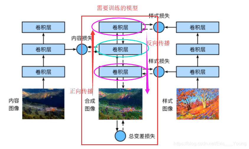

3.2.2.首先，我们初始化合成图像，例如将其初始化成内容图像。
该合成图像是样式迁移过程中唯一需要更新的变量，即样式迁移所需迭代的模型参数
3.2.3.然后，我们选择一个预训练的卷积神经网络来抽取图像的特征，深度卷积神经网络凭借多个层逐级抽取图像的特征。
其中的模型参数在训练中无须更新。
我们可以选择其中某些层的输出作为内容特征或样式特征。例如，选取的预训练的神经网络含有3个卷积层，其中第二层输出图像的内容特征，而第一层和第三层的输出被作为图像的样式特征
3.2.4.接下来，通过正向传播（实线箭头方向）计算样式迁移的损失函数，并通过反向传播（虚线箭头方向）迭代模型参数，即不断更新合成图像。
内容损失（content loss）使合成图像与内容图像在内容特征上接近
样式损失（style loss）令合成图像与样式图像在样式特征上接近，
总变差损失（total variation loss）则有助于减少合成图像中的噪点。
3.2.5.最后，当模型训练结束时，我们输出样式迁移的模型参数，即得到最终的合成图像。

3.3.代码实现

3.3.1.需要导入的包或模块

%matplotlib inline
import time
import torch
import torch.nn.functional as F
import torchvision
import numpy as np
import matplotlib.pyplot as plt
from PIL import Image

import sys
sys.path.append("/home/kesci/input") 
import d2len9900 as d2l
device = torch.device('cuda' if torch.cuda.is_available() else 'cpu') # 均已测试

print(device, torch.__version__)

3.3.2.读取内容图像和样式图像
首先，我们分别读取内容图像和样式图像。从打印出的图像坐标轴可以看出，它们的尺寸并不一样。

#d2l.set_figsize()
content_img = Image.open('/home/kesci/input/NeuralStyle5603/rainier.jpg')
plt.imshow(content_img);

style_img = Image.open('/home/kesci/input/NeuralStyle5603/autumn_oak.jpg')
plt.imshow(style_img);

3.3.3.预处理和后处理图像
预处理函数preprocess对输入图像在RGB三个通道分别做标准化，并将结果变换成卷积神经网络接受的输入格式。
后处理函数postprocess则将输出图像中的像素值还原回标准化之前的值。
由于图像打印函数要求每个像素的浮点数值在0到1之间，我们使用clamp函数对小于0和大于1的值分别取0和1。

rgb_mean = np.array([0.485, 0.456, 0.406])
rgb_std = np.array([0.229, 0.224, 0.225])

def preprocess(PIL_img, image_shape):
    process = torchvision.transforms.Compose([
        torchvision.transforms.Resize(image_shape),
        torchvision.transforms.ToTensor(),
        torchvision.transforms.Normalize(mean=rgb_mean, std=rgb_std)])

    return process(PIL_img).unsqueeze(dim = 0) # (batch_size, 3, H, W)

def postprocess(img_tensor):
    inv_normalize = torchvision.transforms.Normalize(
        mean= -rgb_mean / rgb_std,
        std= 1/rgb_std)
    to_PIL_image = torchvision.transforms.ToPILImage()
    return to_PIL_image(inv_normalize(img_tensor[0].cpu()).clamp(0, 1))

3.3.4.抽取特征
使用基于ImageNet数据集预训练的VGG-19模型来抽取图像特征 ，VGG网络使用了5个卷积块

!echo $TORCH_HOME # 将会把预训练好的模型下载到此处(没有输出的话默认是.cache/torch)
pretrained_net = torchvision.models.vgg19(pretrained=False)
pretrained_net.load_state_dict(torch.load('/home/kesci/input/vgg193427/vgg19-dcbb9e9d.pth'))

一般来说，越靠近输入层的输出越容易抽取图像的细节信息，反之则越容易抽取图像的全局信息。
• 为了避免合成图像过多保留内容图像的细节，我们选择VGG较靠近输出的层，也称内容层，来输出图像的内容特征。实验中，我们选择第四卷积块的最后一个卷积层作为内容层
• 我们还从VGG中选择不同层的输出来匹配局部和全局的样式，这些层也叫样式层。实验中，每个卷积块的第一个卷积层作为样式层
定义两个函数，其中get_contents函数对内容图像抽取内容特征，而get_styles函数则对样式图像抽取样式特征。

def get_contents(image_shape, device):
    content_X = preprocess(content_img, image_shape).to(device)
    contents_Y, _ = extract_features(content_X, content_layers, style_layers)
    return content_X, contents_Y

def get_styles(image_shape, device):
    style_X = preprocess(style_img, image_shape).to(device)
    _, styles_Y = extract_features(style_X, content_layers, style_layers)
    return style_X, styles_Y

• 在训练时无须改变预训练的VGG的模型参数，所以我们可以在训练开始之前就提取出内容图像的内容特征，以及样式图像的样式特征。
在抽取特征时，我们只需要用到VGG从输入层到最靠近输出层的内容层或样式层之间的所有层。下面构建一个新的网络net，它只保留需要用到的VGG的所有层。我们将使用net来抽取特征。

style_layers, content_layers = [0, 5, 10, 19, 28], [25]

net_list = []
for i in range(max(content_layers + style_layers) + 1):
    net_list.append(pretrained_net.features[i])
net = torch.nn.Sequential(*net_list)

• 由于合成图像是样式迁移所需迭代的模型参数，我们只能在训练过程中通过调用extract_features函数来抽取合成图像的内容特征和样式特征。

def extract_features(X, content_layers, style_layers):
    contents = []
    styles = []
    for i in range(len(net)):
        X = net[i](X)
        if i in style_layers:
            styles.append(X)
        if i in content_layers:
            contents.append(X)
    return contents, styles

3.3.5.定义损失函数
内容损失
• 与线性回归中的损失函数类似，内容损失通过平方误差函数衡量合成图像与内容图像在内容特征上的差异。平方误差函数的两个输入均为extract_features函数计算所得到的内容层的输出。

def content_loss(Y_hat, Y):
    return F.mse_loss(Y_hat, Y)

样式损失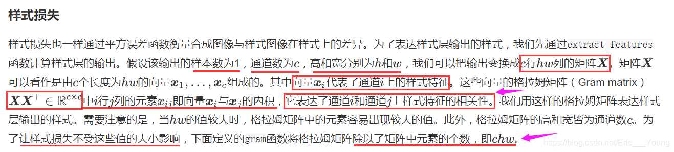

def gram(X):
    num_channels, n = X.shape[1], X.shape[2] * X.shape[3]
    X = X.view(num_channels, n)
    return torch.matmul(X, X.t()) / (num_channels * n)

• 样式损失也一样通过平方误差函数衡量合成图像与样式图像在样式上的差异。为了表达样式层输出的样式，我们先通过extract_features函数计算样式层的输出。
• 样式损失的平方误差函数的两个格拉姆矩阵输入分别基于合成图像与样式图像的样式层输出

def style_loss(Y_hat, gram_Y):
    return F.mse_loss(gram(Y_hat), gram_Y)

总变差损失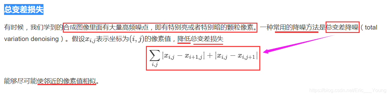

def tv_loss(Y_hat):
    return 0.5 * (F.l1_loss(Y_hat[:, :, 1:, :], Y_hat[:, :, :-1, :]) + 
                  F.l1_loss(Y_hat[:, :, :, 1:], Y_hat[:, :, :, :-1]))

损失函数
• 样式迁移的损失函数即内容损失、样式损失和总变差损失的 加权和。
• 通过调节这些权值超参数，我们可以权衡合成图像在保留内容、迁移样式以及降噪三方面的相对重要性。

content_weight, style_weight, tv_weight = 1, 1e3, 10

def compute_loss(X, contents_Y_hat, styles_Y_hat, contents_Y, styles_Y_gram):
    # 分别计算内容损失、样式损失和总变差损失
    contents_l = [content_loss(Y_hat, Y) * content_weight for Y_hat, Y in zip(
        contents_Y_hat, contents_Y)]
    styles_l = [style_loss(Y_hat, Y) * style_weight for Y_hat, Y in zip(
        styles_Y_hat, styles_Y_gram)]
    tv_l = tv_loss(X) * tv_weight
    # 对所有损失求和
    l = sum(styles_l) + sum(contents_l) + tv_l
    return contents_l, styles_l, tv_l, l

3.3.6.创建和初始化合成图像
在样式迁移中，合成图像是唯一需要更新的变量。因此，我们可以定义一个简单的模型GeneratedImage，并将合成图像视为模型参数。模型的前向计算只需返回模型参数即可。

    def __init__(self, img_shape):
        super(GeneratedImage, self).__init__()
        self.weight = torch.nn.Parameter(torch.rand(*img_shape))

    def forward(self):
        return self.weight

下面，我们定义get_inits函数。该函数创建了合成图像的模型实例，并将其初始化为图像X。样式图像在各个样式层的格拉姆矩阵styles_Y_gram将在训练前预先计算好。

def get_inits(X, device, lr, styles_Y):
    gen_img = GeneratedImage(X.shape).to(device)
    gen_img.weight.data = X.data
    optimizer = torch.optim.Adam(gen_img.parameters(), lr=lr)
    styles_Y_gram = [gram(Y) for Y in styles_Y]
    return gen_img(), styles_Y_gram, optimizer

3.3.7.训练
定义def train函数，在训练模型时，我们不断抽取合成图像的内容特征和样式特征，并计算损失函数。

def train(X, contents_Y, styles_Y, device, lr, max_epochs, lr_decay_epoch):
    print("training on ", device)
    X, styles_Y_gram, optimizer = get_inits(X, device, lr, styles_Y)
    scheduler = torch.optim.lr_scheduler.StepLR(optimizer, lr_decay_epoch, gamma=0.1)
    for i in range(max_epochs):
        start = time.time()
        
        contents_Y_hat, styles_Y_hat = extract_features(
                X, content_layers, style_layers)
        contents_l, styles_l, tv_l, l = compute_loss(
                X, contents_Y_hat, styles_Y_hat, contents_Y, styles_Y_gram)
        
        optimizer.zero_grad()
        l.backward(retain_graph = True)
        optimizer.step()
        scheduler.step()
        
        if i % 50 == 0 and i != 0:
            print('epoch %3d, content loss %.2f, style loss %.2f, '
                  'TV loss %.2f, %.2f sec'
                  % (i, sum(contents_l).item(), sum(styles_l).item(), tv_l.item(),
                     time.time() - start))
    return X.detach()

下面我们开始训练模型。首先将内容图像和样式图像的高和宽分别调整为150和225像素。合成图像将由内容图像来初始化。

image_shape =  (150, 225)
net = net.to(device)
content_X, contents_Y = get_contents(image_shape, device)
style_X, styles_Y = get_styles(image_shape, device)
output = train(content_X, contents_Y, styles_Y, device, 0.01, 500, 200)

下面我们将训练好的合成图像保存起来。可以看到合成图像保留了内容图像的风景和物体，并同时迁移了样式图像的色彩。因为图像尺寸较小，所以细节上依然比较模糊。

plt.imshow(postprocess(output));

为了得到更加清晰的合成图像，下面我们在更大的300X450尺寸上训练。我们将图的高和宽放大2倍，以初始化更大尺寸的合成图像。

image_shape = (300, 450)
_, content_Y = get_contents(image_shape, device)
_, style_Y = get_styles(image_shape, device)
X = preprocess(postprocess(output), image_shape).to(device)
big_output = train(X, content_Y, style_Y, device, 0.01, 500, 200)

plt.imshow(postprocess(big_output));

可以看到，由于图像尺寸更大，每一次迭代需要花费更多的时间。从训练得到的图中可以看到，此时的合成图像因为尺寸更大，所以保留了更多的细节。合成图像里面不仅有大块的类似样式图像的油画色彩块，色彩块中甚至出现了细微的纹理。

3.4.小结

3.4.1.样式迁移常用的损失函数由3部分组成：内容损失使合成图像与内容图像在内容特征上接近，样式损失令合成图像与样式图像在样式特征上接近，而总变差损失则有助于减少合成图像中的噪点。
3.4.2.可以通过预训练的卷积神经网络来抽取图像的特征，并通过最小化损失函数来不断更新合成图像。
3.4.3.用格拉姆矩阵表达样式层输出的样式。