Ceres介绍
- ceres 可以解约束非线性最小二乘问题:

- f i f_ifi:cost function 代价函数,SLAM中叫做误差项
- x j x_jxj:优化变量
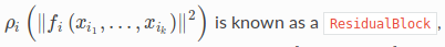
- ρ i \rho_{i}ρi: 核函数
在最简单的情况下:核函数ρ i = x \rho_i=x\space\spaceρi=x 约束条件:l j = − ∞ u j = ∞ l_j=-\infty \space\space u_j=\inftylj=−∞ uj=∞ ,我们得到最熟悉的非线性最小二乘问题:
求解过程
一般利用Ceres求解非线性优化问题分为三个过程:
- 构建代价函数(cost function)
- 通过代价函数来构建优化问题
- 配置求解器
举例叙述
问题:求解 1 2 ( 10 − x ) 2 \frac{1}{2}(10-x)^221(10−x)2的最小值时候的x xx
- 构建代价函数
struct CostFunctor
{
    template <typename T>
    bool operator()(const T* const x, T* residual) const
    {
        residual[0] = T(10.0) - x[0];
        return true;
    }
};
residual:残差(一维)
x:模型参数(一维)
- 构建优化问题
    double initial_x = 5.0;
    double x = initial_x; //变量初始值


    ceres::Problem  problem;
    CostFunction* cost_function = new AutoDiffCostFunction<CostFunctor, 1, 1>(new CostFunctor);
    problem.AddResidualBlock(cost_function, NULL, &x);
(1) 先定义一个求解问题:ceres::Problem problem
(2) 使用自动求导,将之前定义的cost function传入,模板参数:误差类型(自定义的仿函数cost function)、输出维度(残差)、输入维度(变量);顺序与cost function定义相反
(3) 添加误差项: (2)中的cost_function的指针,核函数(NULL不使用),x优化变量
- 配置求解器
    Solver::Options options;
    options.linear_solver_type=DENSE_QR;  //增量方程如何求解
    options.minimizer_progress_to_stdout=true; //迭代过程信息输出到stdout


    Solver::Summary summary; //优化信息
    Solve(options, &problem, &summary); //开始执行求解
求导方法
- Automatic Derivatives(自动求导)
效率比数值求导高
Numeric Derivatives(数值求导)
Analytic Derivatives(解析求导)
曲线拟合
举例
- 拟合y = e x p ( a x 2 + b x + c ) + w y=exp(ax^2+bx+c)+wy=exp(ax2+bx+c)+w
a b c a \space b \space ca b c是曲线参数,w ww是高斯噪声,假设我们有N(100)个带噪声的数据点,拟合曲线,求曲线参数:
min a b c 1 2 ∑ i = 1 N ∣ ∣ y i − e x p ( a x i 2 + b x i + c ) ∣ ∣ 2 \min \limits_{abc} \frac{1}{2}\sum_{i=1}^{N}||y_i-exp(ax_i^2+bx_i+c)||^2abcmin21i=1∑N∣∣yi−exp(axi2+bxi+c)∣∣2
- 定义代价函数
#include <iostream>
#include <opencv4/opencv2/core.hpp>
#include <ceres/ceres.h>
#include <chrono>
#include <fstream>

using namespace std;

//构建代价函数
struct CURVE_FITTING_COST
{
    CURVE_FITTING_COST (double x, double y): _x(x), _y(y) {}

    template<typename T>
    bool operator()(const T* const abc, T* residual) const
    {
        residual[0]=T(_y) - ceres::exp(abc[0]*T(_x) * T(_x) + abc[1]*T(_x) +abc[2]);
        return true;
    }

    const double _x, _y;
};


int main()
{
    string fp("../res/data.txt");
    ofstream outfile;
    outfile.open(fp,ios::trunc);

    double a=1.0, b=2.0, c=1.0; //真实的参数
    int N=100 ;  //数据点
    double w_sigma = 1.0;
    cv::RNG rng;
    double abc[3] = {0,0,0};


    // 数据生成
    vector<double> x_data, y_data;
    cout << "gernerating data" << endl;

    for(int i=0; i<N; i++)
    {
        double x = i/100.0, y=0;
        x_data.push_back(x);
        y = exp(a*x*x+b*x+c)+rng.gaussian(w_sigma);
        y_data.push_back(y);

        outfile << x << "\t"<< y << endl;

        cout << x_data[i] << " " << y_data[i] << endl;
    }


    // 构建最小二乘问题
    ceres::Problem problem;
    for(int i=0; i<N; i++)
    {
        problem.AddResidualBlock(new ceres::AutoDiffCostFunction<CURVE_FITTING_COST, 1, 3>(new CURVE_FITTING_COST(x_data[i], y_data[i])), nullptr, abc);

    }


    //配置优化选项
    ceres::Solver::Options options;
    options.linear_solver_type = ceres::DENSE_QR;
    options.minimizer_progress_to_stdout = true;

    ceres::Solver::Summary summary;
    chrono::steady_clock::time_point t1 = chrono::steady_clock::now();
    ceres::Solve(options, &problem, &summary);//进行优化
    chrono::steady_clock::time_point t2 = chrono::steady_clock::now();

    chrono::duration<double> time_used = chrono::duration_cast<chrono::duration<double>>(t2-t1);
    cout << "solve time cost : " <<  time_used.count()  << "miliseconds" << endl;

    cout << summary.BriefReport() << endl;
    cout << "estimate a,b,c = " ;
    for(auto a:abc)cout << a<< " ";
    cout << endl;

    outfile << abc[0] << "\t"<< abc[1] <<  "\t" << abc[2] << endl;
    outfile.close();
    return 0;
}

估计的参数 a:0.891943 b:2.17039 c:0.944142
原始参数:a: 1 b: 2 b:1
outliers的处理
- 假如有少数极端值(outliers),那么对参数的估计有很大影响,如:

这时候可以借助核函数(loss function)来解决,将
problem.AddResidualBlock(new ceres::AutoDiffCostFunction<CURVE_FITTING_COST, 1, 3>(new CURVE_FITTING_COST(x_data[i], y_data[i])), nullptr, abc);
nullptr 改为 new ceres::CauchyLoss(0.5)
problem.AddResidualBlock(new ceres::AutoDiffCostFunction<CURVE_FITTING_COST, 1, 3>(new CURVE_FITTING_COST(x_data[i], y_data[i])), new ceres::CauchyLoss(0.5), abc);

版权声明:本文为zzyczzyc原创文章,遵循CC 4.0 BY-SA版权协议,转载请附上原文出处链接和本声明。