PCA主成分分析:最广泛无监督算法 + 基础的降维算法。
通过线性变换将原始数据变换为一组各维度线性无关的表示,用于提取数据的主要特征分量 → 高维数据的降维
PCA主成分分析:
二维数据降维 / 多维数据降维 /主成分筛选

二维数据降维
# 加载主成分分析模块PCAfrom sklearn.decomposition import PCA
# 数据创建rng = np.random.RandomState(8)data = np.dot(rng.rand(2,2),rng.randn(2,200)).Tdf = pd.DataFrame({'X1':data[:,0],'X2':data[:,1]})print(rng)print(df.head())print(df.shape)plt.figure(figsize =(10,6))plt.scatter(df['X1'],df['X2'], alpha = 0.8, marker = '.')plt.axis('equal')plt.grid()
RandomState(MT19937)
         X1        X2
0 -1.174787 -1.404131
1 -1.374449 -1.294660
2 -2.316007 -2.166109
3  0.947847  1.460480
4  1.762375  1.640622
(200, 2)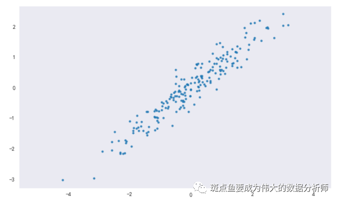
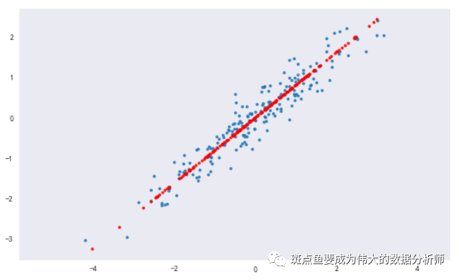
# 构建模型,分析主成分pca = PCA(n_components = 1) # n_components = 1 → 降为1维pca.fit(df) # 构建模型# sklearn.decomposition.PCA(n_components=None, copy=True, whiten=False)# n_components: PCA算法中所要保留的主成分个数n,也即保留下来的特征个数n# copy: True或者False,默认为True → 表示是否在运行算法时,将原始训练数据复制一份# fit(X,y=None) → 调用fit方法的对象本身。比如pca.fit(X),表示用X对pca这个对象进行训练# components_:返回具有最大方差的成分。# explained_variance_ratio_:返回 所保留的n个成分各自的方差百分比。# n_components_:返回所保留的成分个数n。print(pca.explained_variance_) # 输出特征值print(pca.components_) # 输出特征向量print(pca.n_components_) # 输出成分的个数print('-----')# 这里是shape(200,2)降为shape(200,1),只有1个特征值,对应2个特征向量# 降维后主成分 A1 = 0.7788006 * X1 + 0.62727158 * X2# 主成分分析,生成新的向量x_pca# fit_transform(X) → 用X来训练PCA模型,同时返回降维后的数据,这里x_pca就是降维后的数据# inverse_transform() → 将降维后的数据转换成原始数据x_pca = pca.transform(df) # 数据转换x_new = pca.inverse_transform(x_pca) # 将降维后的数据转换成原始数据print(x_new[:10])print(df.head())print('original shape:',df.shape)print('transformed shape:',x_pca.shape)print(x_pca[:5])print('-----')plt.figure(figsize =(10,6))plt.scatter(df['X1'],df['X2'], alpha = 0.8, marker = '.')plt.scatter(x_new[:,0],x_new[:,1], alpha = 0.8, marker = '.',color = 'r')plt.axis('equal')plt.grid()
[2.79699086]
[[-0.7788006  -0.62727158]]
1
-----
[[-1.40189115 -1.12216571]
 [-1.46951341 -1.1766309 ]
 [-2.46631701 -1.97948926]
 [ 1.28496913  1.04191979]
 [ 1.86700832  1.51071326]
 [-0.02329367 -0.01179804]
 [ 1.28199507  1.03952438]
 [ 1.09124665  0.88588933]
 [ 0.01335223  0.01771777]
 [ 3.00384234  2.42635671]]
         X1        X2
0 -1.174787 -1.404131
1 -1.374449 -1.294660
2 -2.316007 -2.166109
3  0.947847  1.460480
4  1.762375  1.640622
original shape: (200, 2)
transformed shape: (200, 1)
[[ 1.77885258]
 [ 1.8656813 ]
 [ 3.14560277]
 [-1.67114513]
[-2.41849842]]![]()
![]()
![]() 多维数据降维
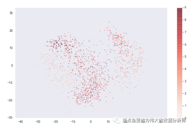
多维数据降维
# 导入数据from sklearn.datasets import load_digitsdigits = load_digits()print(digits .keys())print('数据长度为:%i条' % len(digits['data']))print('数据形状为:%i条',digits.data.shape)print(digits.data[:2])print(digits["target"])
dict_keys(['data', 'target', 'frame', 'feature_names', 'target_names', 'images', 'DESCR'])
数据长度为:1797条
数据形状为:%i条 (1797, 64)
[[ 0.  0.  5. 13.  9.  1.  0.  0.  0.  0. 13. 15. 10. 15.  5.  0.  0.  3.
  15.  2.  0. 11.  8.  0.  0.  4. 12.  0.  0.  8.  8.  0.  0.  5.  8.  0.
   0.  9.  8.  0.  0.  4. 11.  0.  1. 12.  7.  0.  0.  2. 14.  5. 10. 12.
   0.  0.  0.  0.  6. 13. 10.  0.  0.  0.]
 [ 0.  0.  0. 12. 13.  5.  0.  0.  0.  0.  0. 11. 16.  9.  0.  0.  0.  0.
   3. 15. 16.  6.  0.  0.  0.  7. 15. 16. 16.  2.  0.  0.  0.  0.  1. 16.
  16.  3.  0.  0.  0.  0.  1. 16. 16.  6.  0.  0.  0.  0.  1. 16. 16.  6.
   0.  0.  0.  0.  0. 11. 16. 10.  0.  0.]]
[0 1 2 ... 8 9 8]
# 构建模型,分析主成分# 降维后,得到2个成分,每个成分有64个特征向量pca = PCA(n_components = 2) # 降为2纬projected = pca.fit_transform(digits.data)print('original shape:',digits.data.shape)print('transformed shape:',projected.shape)print(pca.explained_variance_) # 输出特征值print(pca.components_.shape) # 输出特征向量形状#print(projected) # 输出解析后数据plt.figure(figsize =(10,6))plt.scatter(projected[:,0],projected[:,1],c = digits.target, edgecolor = 'none',alpha = 0.5,cmap = 'Reds',s = 5)plt.axis('equal')plt.grid()plt.colorbar()

主成分筛选:选取 【贡献率≥85%】 的主成分
# 降维后,得到10个成分,每个成分有64个特征向量pca = PCA(n_components = 10) # 降为10纬projected = pca.fit_transform(digits.data)print('original shape:',digits.data.shape)print('transformed shape:',projected.shape)print(pca.explained_variance_) # 输出特征值print(pca.components_.shape) # 输出特征向量形状#print(projected) # 输出解析后数据c_s = pd.DataFrame({'b':pca.explained_variance_,'b_sum':pca.explained_variance_.cumsum()/pca.explained_variance_.sum()})print(c_s)# 做贡献率累计求和# 可以看到第7个成分时候,贡献率超过85% → 选取前7个成分作为主成分plt.figure(figsize =(10,8))c_s['b_sum'].plot(style = '--ko', figsize = (10,4))plt.axhline(0.85,color='r',linestyle="--",alpha=0.8)plt.text(6,c_s['b_sum'].iloc[6]-0.08,'第7个成分累计贡献率超过85%',color = 'r')plt.grid()
original shape: (1797, 64)
transformed shape: (1797, 10)
[179.00693009 163.71774688 141.78843904 101.10037476  69.51316464
  59.10849686  51.88452824  44.0148488   40.31087091  37.01129311]
(10, 64)
            b     b_sum
0  179.006930  0.201708
1  163.717747  0.386187
2  141.788439  0.545957
3  101.100375  0.659878
4   69.513165  0.738207
5   59.108497  0.804811
6   51.884528  0.863276
7   44.014849  0.912872
8   40.310871  0.958295
9   37.011293  1.000000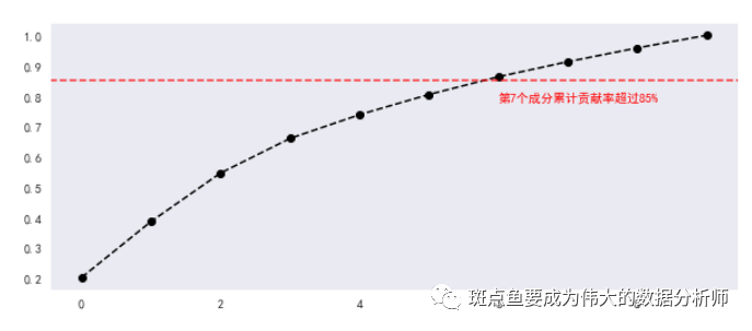
版权声明:本文为weixin_40637477原创文章,遵循CC 4.0 BY-SA版权协议,转载请附上原文出处链接和本声明。