SoftMax回归 http://ufldl.stanford.edu/wiki/index.php/Softmax%E5%9B%9E%E5%BD%92
我们的训练集由  个已标记的样本构成:
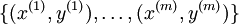 ,其中输入特征
 。(我们对符号的约定如下:特征向量
  的维度为
的维度为  ,其中
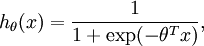
,其中  对应截距项 。) 由于 logistic 回归是针对二分类问题的,因此类标记
  。假设函数(hypothesis function) 如下:
我们将训练模型参数  ,使其能够最小化代价函数 :
![\begin{align} J(\theta) = -\frac{1}{m} \left[ \sum_{i=1}^m y^{(i)} \log h_\theta(x^{(i)}) + (1-y^{(i)}) \log (1-h_\theta(x^{(i)})) \right] \end{align}](http://ufldl.stanford.edu/wiki/images/math/f/a/6/fa6565f1e7b91831e306ec404ccc1156.png)
在 softmax回归中,我们解决的是多分类问题(相对于 logistic 回归解决的二分类问题),类标  可以取
可以取  个不同的值(而不是 2 个)。因此,对于训练集 ,我们有
 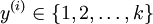 。(注意此处的类别下标从 1 开始,而不是 0)。例如,在 MNIST 数字识别任务中,我们有
  个不同的类别。
对于给定的测试输入 ,我们想用假设函数针对每一个类别j估算出概率值  。也就是说,我们想估计 的每一种分类结果出现的概率。因此,我们的假设函数将要输出一个 维的向量(向量元素的和为1)来表示这 个估计的概率值。 具体地说,我们的假设函数
  形式如下:
形式如下:
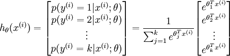
其中 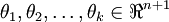 是模型的参数。请注意
  这一项对概率分布进行归一化,使得所有概率之和为 1 。
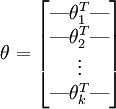
为了方便起见,我们同样使用符号 来表示全部的模型参数。在实现Softmax回归时,将 用一个  的矩阵来表示会很方便,该矩阵是将
  按行罗列起来得到的,如下所示:
代价函数
现在我们来介绍 softmax 回归算法的代价函数。在下面的公式中, 是示性函数,其取值规则为:
 值为真的表达式
  , 值为假的表达式
  。举例来说,表达式
  的值为1 ,
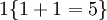 的值为 0。我们的代价函数为:
![\begin{align} J(\theta) = - \frac{1}{m} \left[ \sum_{i=1}^{m} \sum_{j=1}^{k} 1\left\{y^{(i)} = j\right\} \log \frac{e^{\theta_j^T x^{(i)}}}{\sum_{l=1}^k e^{ \theta_l^T x^{(i)} }}\right] \end{align}](http://ufldl.stanford.edu/wiki/images/math/7/6/3/7634eb3b08dc003aa4591a95824d4fbd.png)
值得注意的是,上述公式是logistic回归代价函数的推广。logistic回归代价函数可以改为:
![\begin{align} J(\theta) &= -\frac{1}{m} \left[ \sum_{i=1}^m (1-y^{(i)}) \log (1-h_\theta(x^{(i)})) + y^{(i)} \log h_\theta(x^{(i)}) \right] \\ &= - \frac{1}{m} \left[ \sum_{i=1}^{m} \sum_{j=0}^{1} 1\left\{y^{(i)} = j\right\} \log p(y^{(i)} = j | x^{(i)} ; \theta) \right] \end{align}](http://ufldl.stanford.edu/wiki/images/math/5/4/9/5491271f19161f8ea6a6b2a82c83fc3a.png)
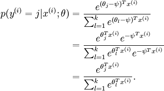
可以看到,Softmax代价函数与logistic 代价函数在形式上非常类似,只是在Softmax损失函数中对类标记的 个可能值进行了累加。注意在Softmax回归中将 分类为类别  的概率为:
的概率为:
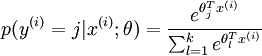 .
.
对于  的最小化问题,目前还没有闭式解法。因此,我们使用迭代的优化算法(例如梯度下降法,或 L-BFGS)。经过求导,我们得到梯度公式如下:
![\begin{align} \nabla_{\theta_j} J(\theta) = - \frac{1}{m} \sum_{i=1}^{m}{ \left[ x^{(i)} \left( 1\{ y^{(i)} = j\} - p(y^{(i)} = j | x^{(i)}; \theta) \right) \right] } \end{align}](http://ufldl.stanford.edu/wiki/images/math/5/9/e/59ef406cef112eb75e54808b560587c9.png)
让我们来回顾一下符号 " " 的含义。
 本身是一个向量,它的第
  个元素
个元素  是 对
是 对 的第 个分量的偏导数。
有了上面的偏导数公式以后,我们就可以将它代入到梯度下降法等算法中,来最小化 。 例如,在梯度下降法的标准实现中,每一次迭代需要进行如下更新: 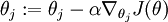 (
( )。
)。
当实现 softmax 回归算法时, 我们通常会使用上述代价函数的一个改进版本。具体来说,就是和权重衰减(weight decay)一起使用。我们接下来介绍使用它的动机和细节。
Softmax回归模型参数化的特点
Softmax 回归有一个不寻常的特点:它有一个“冗余”的参数集。为了便于阐述这一特点,假设我们从参数向量 中减去了向量  ,这时,每一个 都变成了
  ()。此时假设函数变成了以下的式子:
换句话说,从 中减去 完全不影响假设函数的预测结果!这表明前面的 softmax 回归模型中存在冗余的参数。更正式一点来说, Softmax 模型被过度参数化了。对于任意一个用于拟合数据的假设函数,可以求出多组参数值,这些参数得到的是完全相同的假设函数  。
。
进一步而言,如果参数  是代价函数 的极小值点,那么
  同样也是它的极小值点,其中 可以为任意向量。因此使 最小化的解不是唯一的。(有趣的是,由于 仍然是一个凸函数,因此梯度下降时不会遇到局部最优解的问题。但是 Hessian 矩阵是奇异的/不可逆的,这会直接导致采用牛顿法优化就遇到数值计算的问题)
注意,当  时,我们总是可以将
  替换为
替换为 (即替换为全零向量),并且这种变换不会影响假设函数。因此我们可以去掉参数向量 (或者其他 中的任意一个)而不影响假设函数的表达能力。实际上,与其优化全部的 个参数 (其中
  ),我们可以令
  ,只优化剩余的
  个参数,这样算法依然能够正常工作。
在实际应用中,为了使算法实现更简单清楚,往往保留所有参数  ,而不任意地将某一参数设置为 0。但此时我们需要对代价函数做一个改动:加入权重衰减。权重衰减可以解决 softmax 回归的参数冗余所带来的数值问题。
权重衰减
我们通过添加一个权重衰减项 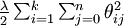 来修改代价函数,这个衰减项会惩罚过大的参数值,现在我们的代价函数变为:
![\begin{align} J(\theta) = - \frac{1}{m} \left[ \sum_{i=1}^{m} \sum_{j=1}^{k} 1\left\{y^{(i)} = j\right\} \log \frac{e^{\theta_j^T x^{(i)}}}{\sum_{l=1}^k e^{ \theta_l^T x^{(i)} }} \right] + \frac{\lambda}{2} \sum_{i=1}^k \sum_{j=0}^n \theta_{ij}^2 \end{align}](http://ufldl.stanford.edu/wiki/images/math/4/7/1/471592d82c7f51526bb3876c6b0f868d.png)
有了这个权重衰减项以后 ( ),代价函数就变成了严格的凸函数,这样就可以保证得到唯一的解了。 此时的 Hessian矩阵变为可逆矩阵,并且因为是凸函数,梯度下降法和 L-BFGS 等算法可以保证收敛到全局最优解。
为了使用优化算法,我们需要求得这个新函数 的导数,如下:
![\begin{align} \nabla_{\theta_j} J(\theta) = - \frac{1}{m} \sum_{i=1}^{m}{ \left[ x^{(i)} ( 1\{ y^{(i)} = j\} - p(y^{(i)} = j | x^{(i)}; \theta) ) \right] } + \lambda \theta_j \end{align}](http://ufldl.stanford.edu/wiki/images/math/3/a/f/3afb4b9181a3063ddc639099bc919197.png)
通过最小化 ,我们就能实现一个可用的 softmax 回归模型。
Softmax回归与Logistic 回归的关系
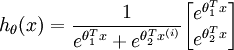
当类别数  时,softmax 回归退化为 logistic 回归。这表明 softmax 回归是 logistic 回归的一般形式。具体地说,当 时,softmax 回归的假设函数为:
利用softmax回归参数冗余的特点,我们令 ,并且从两个参数向量中都减去向量 ,得到:
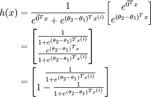
因此,用  来表示
来表示 ,我们就会发现 softmax 回归器预测其中一个类别的概率为
  ,另一个类别概率的为
 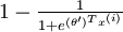 ,这与 logistic回归是一致的。
input_data代码
# Copyright 2015 The TensorFlow Authors. All Rights Reserved.
#
# Licensed under the Apache License, Version 2.0 (the "License");
# you may not use this file except in compliance with the License.
# You may obtain a copy of the License at
#
#     http://www.apache.org/licenses/LICENSE-2.0
#
# Unless required by applicable law or agreed to in writing, software
# distributed under the License is distributed on an "AS IS" BASIS,
# WITHOUT WARRANTIES OR CONDITIONS OF ANY KIND, either express or implied.
# See the License for the specific language governing permissions and
# limitations under the License.
# ==============================================================================

"""Functions for downloading and reading MNIST data."""
from __future__ import absolute_import
from __future__ import division
from __future__ import print_function

import gzip
import os
import tempfile

import numpy
from six.moves import urllib
from six.moves import xrange  # pylint: disable=redefined-builtin
import tensorflow as tf
from tensorflow.contrib.learn.python.learn.datasets.mnist import read_data_sets
TensorFlow代码:
# coding:utf-8
import input_data
import tensorflow as tf
mnist = input_data.read_data_sets("Image/", one_hot=True)
x=tf.placeholder(tf.float32,[None,784]) #创建存储样本的表
W=tf.Variable(tf.zeros([784,10])) #创建变换矩阵W
b=tf.Variable(tf.zeros([10])) #创建偏置常量b
#学习的是W与b
y=tf.nn.softmax(tf.matmul(x,W)+b)#设置好模型放入softmax回归函数中
y_=tf.placeholder("float",[None,10])#用于存储真是的数据标签
#利用交叉熵作为coastFunction
cross_entropy=-tf.reduce_sum(y_*tf.log(y))
#利用梯度下降方法最小化coastFunction
train_step=tf.train.GradientDescentOptimizer(0.01).minimize(cross_entropy)
#初始化所有变量
init=tf.global_variables_initializer()
sess=tf.Session()
sess.run(init)
for i in range(1000):
    #每次随机抓取100个数据点进行训练
    bach_xs,bach_ys=mnist.train.next_batch(100)
    sess.run(train_step,feed_dict={x:bach_xs,y_:bach_ys})
#训练结束
#计算精度
#tf.equal 该函数计算矩阵对应元素相等 返回对比结果返回布尔值  argmax返回最大值的索引
correct_prediction=tf.equal(tf.argmax(y,1),tf.argmax(y_,1))
#tf.cast把布尔转化为float
accuracy=tf.reduce_mean(tf.cast(correct_prediction,"float"))
#输出结果
print sess.run(accuracy,feed_dict={x:mnist.test.images,y_:mnist.test.labels})
转载于:https://www.cnblogs.com/zhaiyansheng/p/7571647.html