(a)
(1)
(2)
For the sake of simplicity, it is rewritten as the following canonial form :
(0)
(1)
(2)
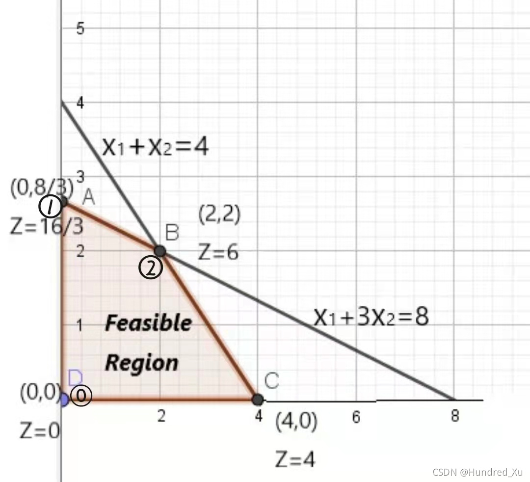
(b) is a CPF solution of the original model;
is the corresponding augmented solution(a basic feasible solution).
are the nonbasic variables;
are the basic variables.
is a CPF solution of the original model;
is the corresponding augmented solution(a basic feasible solution).
are the nonbasic variables;
are the basic variables.
is a CPF solution of the original model;
is the corresponding augmented solution(a basic feasible solution).
are the nonbasic variables;
are the basic variables.
is a CPF solution of the original model;
is the corresponding augmented solution(a basic feasible solution).
are the nonbasic variables;
are the basic variables.
(c)
,
When the nonbasic variables are set equal to zero,this BF solution also is the simultaneous solution of the system of equations obtained in part (a).
,
When the nonbasic variables are set equal to zero,this BF solution also is the simultaneous solution of the system of equations obtained in part (a).
,
When the nonbasic variables are set equal to zero,this BF solution also is the simultaneous solution of the system of equations obtained in part (a).
,
When the nonbasic variables are set equal to zero,this BF solution also is the simultaneous solution of the system of equations obtained in part (a).
(d) is the corner-point infeasible solution;
is the corresponding basic infeasible solution.
are the nonbasic variables;
are the basic variables.
is the corner-point infeasible solution;
is the corresponding basic infeasible solution.
are the nonbasic variables;
are the basic variables.
(e),
When the nonbasic variables are set equal to zero,this BF solution also is the simultaneous solution of the system of equations obtained in part (a).
,
When the nonbasic variables are set equal to zero,this BF solution also is the simultaneous solution of the system of equations obtained in part (a).

Initialization (Iteration 0)
Set and
be the non-basic variables and the other variables are set to be the basic variables. Then we obtain the values of the basic variables
and hence we have the initial BF solution
.
Optimality Test
At the initial BF solution, .
Obviously,increasing the values of or
can bring an improvement to Z. So, the current BF solution is NOT optimal.
Iteration 1
1.Determining Where to Go
Choose the non-basic variable with largest improvement in Z.
Increasing this non-basic variable from zero will convert it to a basic variable for the next BF solution. It is called the entering (basic) variable for iteration 1.
Prototype Example :
Objective function :
Rate of improvement in Z by increasing
Rate of improvement in Z by increasing
Thus, we should choose .
2.Determining Where to Stop
Increasing
increases Z , so we want to go as far as possible without leaving the feasible region.
Minimum Ratio Test :
To identify the maximum possible improvement we can make with which we still inside the feasible region.
Non-basic variable : =0
(1):
(2):
These implies, . Therefore, we set
.
When , eq.(1) gives
and leaves the basis. (
is called the leaving (basic) variable for iteration 1.)
3.Solving for the New BF Solution
The purpose of step 3 is to convert the system of equations to the canonical form. The solution can then be read easily.
By elementary row operations, we solve the system of equations for
:
New eq.(1)=eq.(1)/3
New eq.(0)=eq.(0)+2eq.(1)
New eq.(2)=eq.(2) - New eq.(1)
The resulting canonical form of the model is:
(0)
(1)
(2)
Since
and
are non-basic variables, thus
and
and hence the new BF solution,
, which yields
.
Optimality Test
The current eq.(0) gives the current objective function:
Such has a positive coeffiicient, increasing
would lead to an adjacent BF solution that is better than the current BF soution, so the current solution is NOT optimal.
Iteration 2
1.Determining Where to Go
Now , Z can be increased by increasing
, but not
. Therefore, we choose
as the entering variable.
2.Determining Where to Stop (Minimun Ratio Test)
Non-basic Variable:
(1):
(2):
By the minimum ratio test, we conclude that we should choose as the leaving variable and should set
.
3.Solving for the New BF Solution
New eq.(2)=eq.(1)/2-eq.(2)/2
New eq.(1)=New eq.(2)-eq.(1)
New eq.(0)=eq.(0)+New eq.(1)+2New eq.(2)
The resulting canonical form of the model is:
(0)
(1)
(2)
The new BF solution is and the corresponding
.
Optimality Test
Since increasing the non-basic variables ( and
) would not increase Z, the current BF solution is optimal. The optimal BF solution is
, which implies the optimal solution to the original problem is
and the corresponding optimal value
.
Initialization (Iteration 0)
| bv | Z | rhs | |
| Z | 1 | -1 -2 0 0 | 0 |
0 0 | 1 3 1 0 1 1 0 1 | 8 4 |
Optimality Test
The current BF solution is optimal if and only if every coefficient in row 0 is non-negative.
Now, the coefficient of both
and
in row 0 are negative, therefore the current BF solution is NOT optimal.
Iteration 1
1.Determining the Entering Variable (Determining Where to Go)
Select the non-basic variable with the "most negative" coefficient. The column below this coefficient is called the pivot column.
| bv | Z | rhs | |
| Z | 1 | -1 -2 0 0 | 0 |
0 0 | 1 3 1 0 1 1 0 1 | 8 4 |
2.Determining the Leaving Variable by the Minimum Ratio Test (Determining Where to Stop)
Pick up the strictly positive coefficient in the pivot column and then calculate "rhs / value of pivot column's element".
Choose the variable with the minimum value of the ratio as the leaving variable. The row is called the pivot row.
| bv | Z | rhs | ratio | |
| Z | 1 | -1 -2 0 0 | 0 | |
0 0 | 1 3 1 0 1 1 0 1 | 8 4 | 8/3=8/3 4/1=4 |
3.Solving for the New BF Solution
Create a coefficient 1 for the entering variable in the pivot row by multiplying the row by a suitable number.
Create a coefficient 0 for the entering variable in all rows except the pivot row by adding a suitable multiple of the pivot row.
| bv | Z | rhs | |
| Z | 1 | -1/3 0 2/3 0 | 16/3 |
0 0 | 1/3 1 1/3 0 2/3 0 -1/3 1 | 8/3 4/3 |
Optimality Test
The coefficient of in row 0 is negative, therefore the current BF solution is NOT optimal.
Iteration 2
| bv | Z | rhs | ratio | |
| Z | 1 | -1/3 0 2/3 0 | 0 | |
0 0 | 1/3 1 1/3 0 2/3 0 1/3 1 | 8/3 4/3 | (8/3)/(1/3)=8 (4/3)/(2/3)=2 |
| bv | Z | rhs | |
| Z | 1 | 0 1/2 0 1/2 | 6 |
0 0 | 1 0 -1/2 3/2 0 1 1/2 -1/2 | 2 2 |
Optimality Test
Since none of the coefficient in row 0 are negative, the current BF solution is optimal.
The optimal BF solution is , which implies the optimal solution to the original is
and the corresponding
.
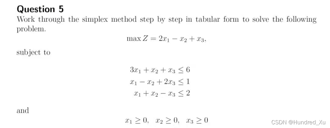
Initialization (Iteration 0)
| bv | Z | rhs | |
| Z | 1 | -2 1 -1 0 0 0 | 0 |
0 0 0 | 3 1 1 1 0 0 1 -1 2 0 1 0 1 1 -1 0 0 1 | 6 1 2 |
Optimality Test
The current BF solution is optimal if and only if every coefficient in row 0 is non-negative.
Now, the coefficient of both
and
in row 0 are negative, therefore the current BF solution is NOT optimal.
Iteration 1
1.Determining the Entering Variable (Determining Where to Go)
Select the non-basic variable with the "most negative" coefficient. The column below this coefficient is called the pivot column.
| bv | Z | rhs | |
| Z | 1 | -2 1 -1 0 0 0 | 0 |
0 0 0 | 3 1 1 1 0 0 1 -1 2 0 1 0 1 1 -1 0 0 1 | 6 1 2 |
2.Determining the Leaving Variable by the Minimum Ratio Test (Determining Where to Stop)
Pick up the strictly positive coefficient in the pivot column and then calculate "rhs / value of pivot column's element".
Choose the variable with the minimum value of the ratio as the leaving variable. The row is called the pivot row.
| bv | Z | rhs | ratio | |
| Z | 1 | -2 1 -1 0 0 0 | 0 | |
0 0 0 | 3 1 1 1 0 0 1 -1 2 0 1 0 1 1 -1 0 0 1 | 6 1 2 | 6/3=2 1/1=1 2/1=2 |
3.Solving for the New BF Solution
Create a coefficient 1 for the entering variable in the pivot row by multiplying the row by a suitable number.
Create a coefficient 0 for the entering variable in all rows except the pivot row by adding a suitable multiple of the pivot row.
| bv | Z | rhs | |
| Z | 1 | 0 -1 3 0 2 0 | 2 |
0 0 0 | 0 4 -5 1 -3 0 1 -1 2 0 1 0 0 2 -3 0 -1 1 | 3 1 1 |
Optimality Test
The coefficient of in row 0 is negative, therefore the current BF solution is NOT optimal.
Iteration 2
| bv | Z | rhs | ratio | |
| Z | 1 | 0 -1 3 0 2 0 | 2 | |
0 0 0 | 0 4 -5 1 -3 0 1 -1 2 0 1 0 0 2 -3 0 -1 1 | 3 1 1 | 3/4=3/4 1/2=1/2 |
| bv | Z | rhs | |
| Z | 1 | 0 0 3/2 0 3/2 1/2 | 5/2 |
0 0 0 | 0 0 1 1 1 -2 1 0 1/2 0 1/2 1/2 0 1 -3/2 0 -1/2 1/2 | 1 3/2 1/2 |
Optimality Test
Since none of the coefficient in row 0 are negative, the current BF solution is optimal.
The optimal BF solution is , which implies the optimal solution to the original is
and the corresponding
.