MATLAB绘图基础
2 MATLAB的立体绘图
2.1 生成网格坐标矩阵的函数
| [X,Y]=meshgrid(x,y) | 生成X-Y平面的网格坐标矩阵 |
|---|---|
| [X,Y,Z]=sphere(n) | 生成球面的三维坐标矩阵 |
| [X,Y,Z]=cylinder(r,n) | 生成柱面的三维坐标矩阵 |
| [X,Y]=meshgrid(x,y);Z=peaks(X,Y) | peaks多峰函数,生成多峰曲面的坐标矩阵 |
例子:
%例一
theta=0:pi/50:6*pi;
x=cos(theta); y=sin(theta); z=0:300;
plot3(x,y,z);
%例二
x=-3:0.1:3; y=-3:0.1:3;
[X,Y]=meshgrid(x,y); Z=X.^2+Y.^2;
surf(X,Y,Z);
2.2 画三维曲面的函数
| plot3(X,Y,Z) | 三维曲面 |
|---|---|
| mesh(X,Y,Z) | 三维网格曲面 |
| meshz(X,Y,Z) | 可将曲面加上围裙 |
| meshc(X,Y,Z) | 同时画出网状图与等高线 |
| surf(X,Y,Z) | 三维填充曲面(更精细) |
| surfc(X,Y,Z) | 同时画出曲面图与等高线 |
| bar3(A) | 三维柱状图 |
| stem3(A) | 三维棒状图 |
| pie3(A) | 三维饼状图 |
| fill3(A) | 三维填充图 |
| waterfall(X,Y,Z) | 三维瀑布图,可在x方向或y方向产生水流效果 |
| contour3(X,Y,Z) | 三维等高线图 |
| contour(X,Y,Z) | 画出曲面等高线在XY平面的投影 |
例子:
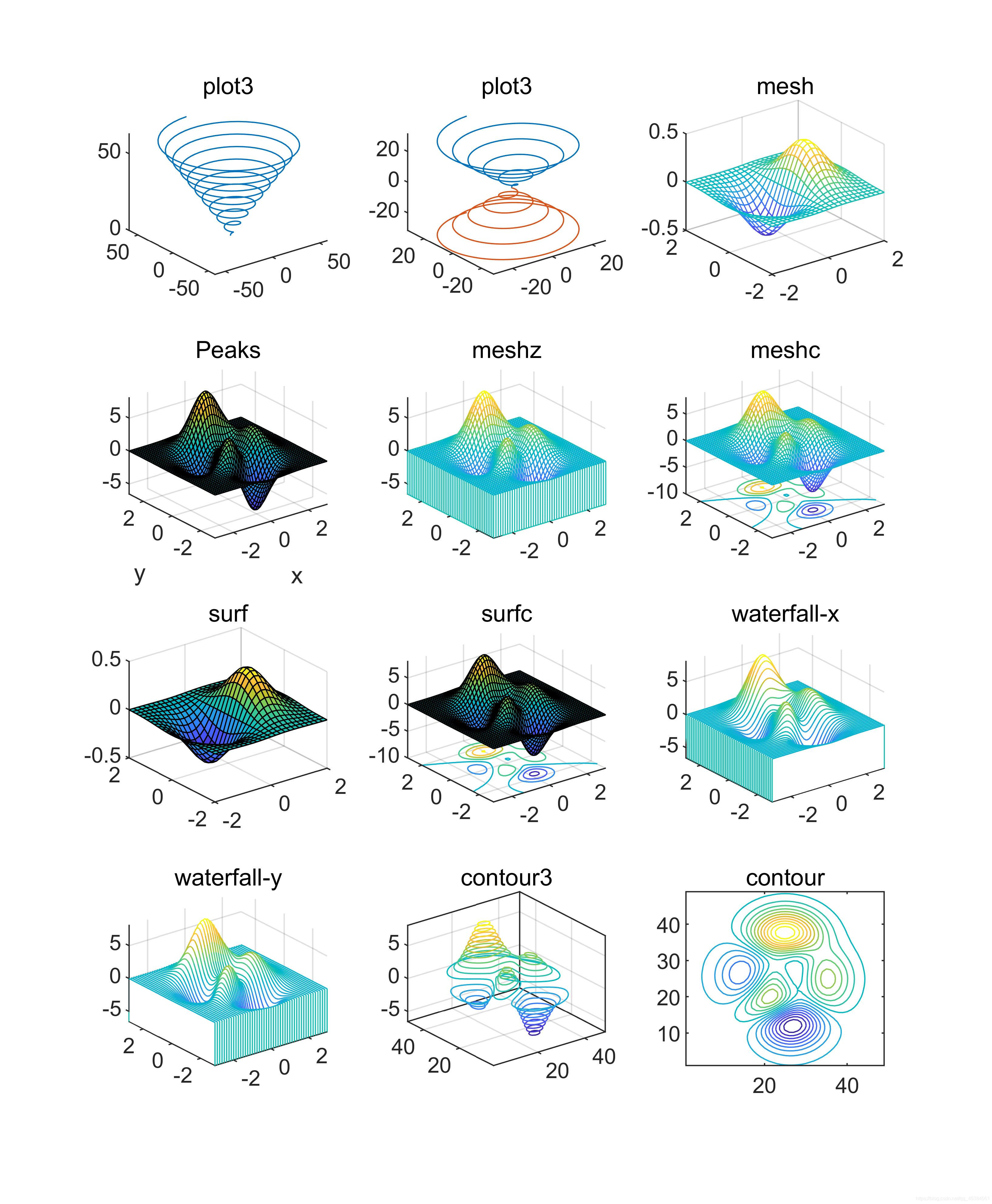
%mesh和plot是三度空间立体绘图的基本命令,mesh可画出立体网状图,plot则可画出立体曲面图,两者产生的图形都会依高度而有不同颜色。
%plot3可画出三度空间中的曲线。
t=linspace(0,20*pi, 501);
subplot(3,4,1),plot3(t.*sin(t), t.*cos(t), t);title('plot3');
%也可同时画出两条三度空间中的曲线
t=linspace(0, 10*pi, 501);
subplot(3,4,2),plot3(t.*sin(t), t.*cos(t), t, t.*sin(t), t.*cos(t), -t);title('plot3');
%mesh可画出立体网状图。
x=linspace(-2, 2, 25); %在x轴上取25点
y=linspace(-2, 2, 25); %在y轴上取25点
[xx,yy]=meshgrid(x, y); %xx和yy都是21x21的矩阵
zz=xx.*exp(-xx.^2-yy.^2); %计算函数值,zz也是21x21的矩阵
subplot(3,4,3),mesh(xx, yy, zz);title('mesh'); %画出立体网状图
%peaks函数可产生一个凹凸有致的曲面,包含了三个局部极大点及三个局部极小点。
subplot(3,4,4),peaks;
%meshz可将曲面加上围裙。
[x,y,z]=peaks;
subplot(3,4,5),meshz(x,y,z);title('meshz');
axis([-inf inf -inf inf -inf inf]);
%meshc同时画出网状图与等高线。
[x,y,z]=peaks;
subplot(3,4,6),meshc(x,y,z);title('meshc');
axis([-inf inf -inf inf -inf inf]);
%surf画出立体曲面图
x=linspace(-2, 2, 25); %在x轴上取25点
y=linspace(-2, 2, 25); %在y轴上取25点
[xx,yy]=meshgrid(x, y); %xx和yy都是21x21的矩阵
zz=xx.*exp(-xx.^2-yy.^2); %计算函数值,zz也是21x21的矩阵
subplot(3,4,7),surf(xx, yy, zz);title('surf'); %画出立体曲面图
%surfc同时画出曲面图与等高线。
[x,y,z]=peaks;
subplot(3,4,8),surfc(x,y,z);title('surfc');
axis([-inf inf -inf inf -inf inf]);
%waterfall可在x方向或y方向产生水流效果。
[x,y,z]=peaks;
subplot(3,4,9),waterfall(x,y,z);title('waterfall-x');
axis([-inf inf -inf inf -inf inf]);
%在y方向产生水流效果
[x,y,z]=peaks;
subplot(3,4,10),waterfall(x',y',z');title('waterfall-y');
axis([-inf inf -inf inf -inf inf]);
%contour3画出曲面在三度空间中的等高线。
subplot(3,4,11),contour3(peaks, 20);title('contour3');
axis([-inf inf -inf inf -inf inf]);
%contour画出曲面等高线在XY平面的投影。
subplot(3,4,12),contour(peaks, 20);title('contour');
2.3 三维旋转体的绘制
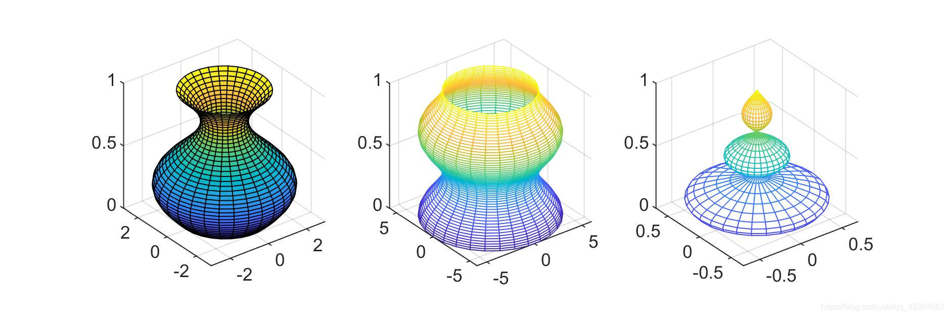
柱面图
由cylinder函数实现,调用格式为:
[x,y,z]=cylinder(R,n); %其中R是一个向量,存放柱面各个等间隔高度上的半径,n表示在圆柱圆周上有n个间隔点,默认有20个间隔点。
如:cylinder(3)生成一个圆柱,cylinder([10,1])生成一个圆锥,而t=0:pi/100:4*pi; R=sin(t); cylinder(R,30);生成一个正弦圆柱面。
[X,Y,Z]=cylinder(R)或[X,Y,Z]=cylinder此形式为默认N=20且R=[1 1]
例子:
t=0:pi/20:2*pi;
[x,y,z]=cylinder(2+sin(t),30);
subplot(1,3,1);surf(x,y,z);
axis('equal');axis('square'); %控制坐标轴的大小相同
subplot(1,3,2);
x=0:pi/20:pi*3;
r=5+cos(x);
[a,b,c]=cylinder(r,30);
mesh(a,b,c);
axis('equal');axis('square');
subplot(1,3,3);
r=abs(exp(-0.25*t).*sin(t));
t=0:pi/12:3*pi;
r=abs(exp(-0.25*t).*sin(t));
[X,Y,Z]=cylinder(r,30);
mesh(X,Y,Z);
colormap([1 0 0]);
axis('equal');axis('square');
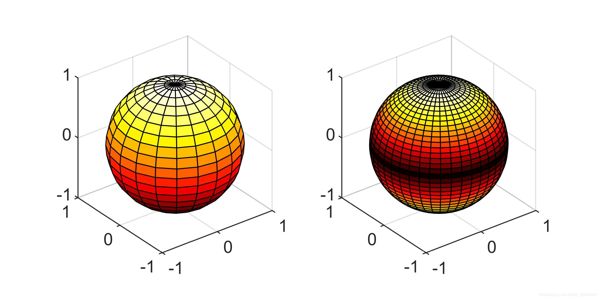
球面图
由sphere函数实现,调用格式为:
[X,Y,Z]=sphere(N); %此函数生成3个(N+1)*(N+1)的矩阵,利用函数surf(X,Y,Z) 可绘制出圆心位于原点、半径为1的单位球体。
n决定了球面的圆滑程度,其默认值为20。若n值取的比较小,则绘制出多面体的表面图。
[X,Y,Z]=sphere; %此形式使用了默认值N=20。
sphere(N); %只是绘制了球面图而不返回任何值。
例子:
subplot(1,2,1);
[x,y,z]=sphere;
surf(x,y,z);
axis('equal');axis('square'); %控制坐标轴的大小相同
subplot(1,2,2);
[a,b,c]=sphere(40);
t=abs(c);
surf(a,b,c,t);
axis('equal');axis('square');
colormap('hot');
2.4 三维图形的处理
视点处理
设置视点的函数view,调用格式为:
view(az,el); %其中az为方位角,el为仰角,它们均以度为单位。系统默认的视点定义为方位角为-37.5度,仰角30度。
例子:
subplot(2,2,1);mesh(peaks);view(-37.5,30);title('-37.5°,30°');
subplot(2,2,2);mesh(peaks);view(0,90);title('0°,90°');
subplot(2,2,3);mesh(peaks);view(90,0);title('90°,0°');
subplot(2,2,4);mesh(peaks);view(-7,-10);title('-7°,-10°');

色彩处理
内建矩阵
colormap hot
三维图形表面的着色
shading faceted; %将每个网格片用其高度对应的颜色进行着色,网格线是黑色
shading flat; %将每个网格片用同一个颜色进行着色,且网格线也用相应的颜色
shading interp; %在网格片内采用颜色插值处理
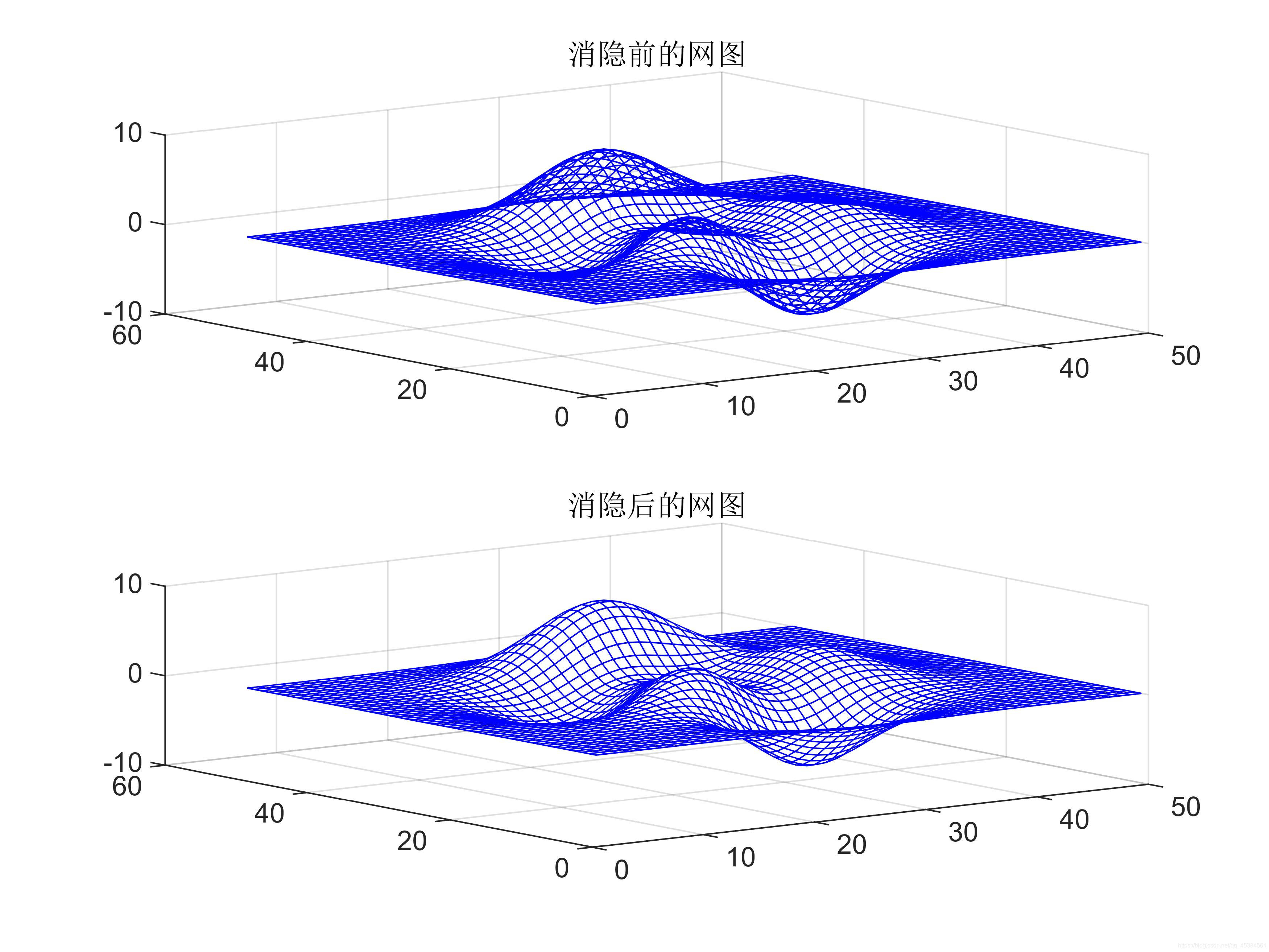
消隐处理
例子:
z=peaks(50);
subplot(2,1,1);
mesh(z);title('消隐前的网图')
hidden off
subplot(2,1,2)
mesh(z);title('消隐后的网图')
hidden on
colormap([0 0 1]);
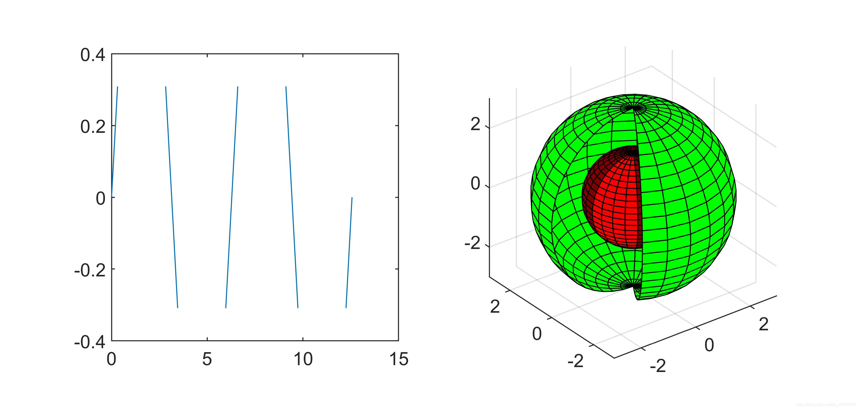
裁剪处理
将图形中需要裁剪部分对应的函数值设置成NaN,使函数值为NaN的部分将不显示出来,从而达到对图形进行裁剪的目的。
例子:
%削掉正弦波顶部或底部大于0.5的部分。
subplot(1,2,1);
x=0:pi/10:4*pi;
y=sin(x);
i=find(abs(y)>0.5);
x(i)=NaN;
plot(x,y);
axis([0 15 -0.4 0.4]);axis square
%绘制两个球面,其中一个在另一个里面,将外面的球裁掉一部分,以便能看到里面的球。
subplot(1,2,2);
[x,y,z]=sphere(25);%生成外面的大球
z1=z;
z1(:,1:4)=NaN;%将大球裁去一部分
c1=ones(size(z1));
surf(3*x,3*y,3*z1,c1);       %生成里面的小球
hold on
z2=z;
c2=2*ones(size(z2));
c2(:,1:4)=3*ones(size(c2(:,1:4)));
surf(1.5*x,1.5*y,1.5*z2,c2);
colormap([0 1 0;0.5 0 0;1 0 0]);
grid on;hold off;axis equal
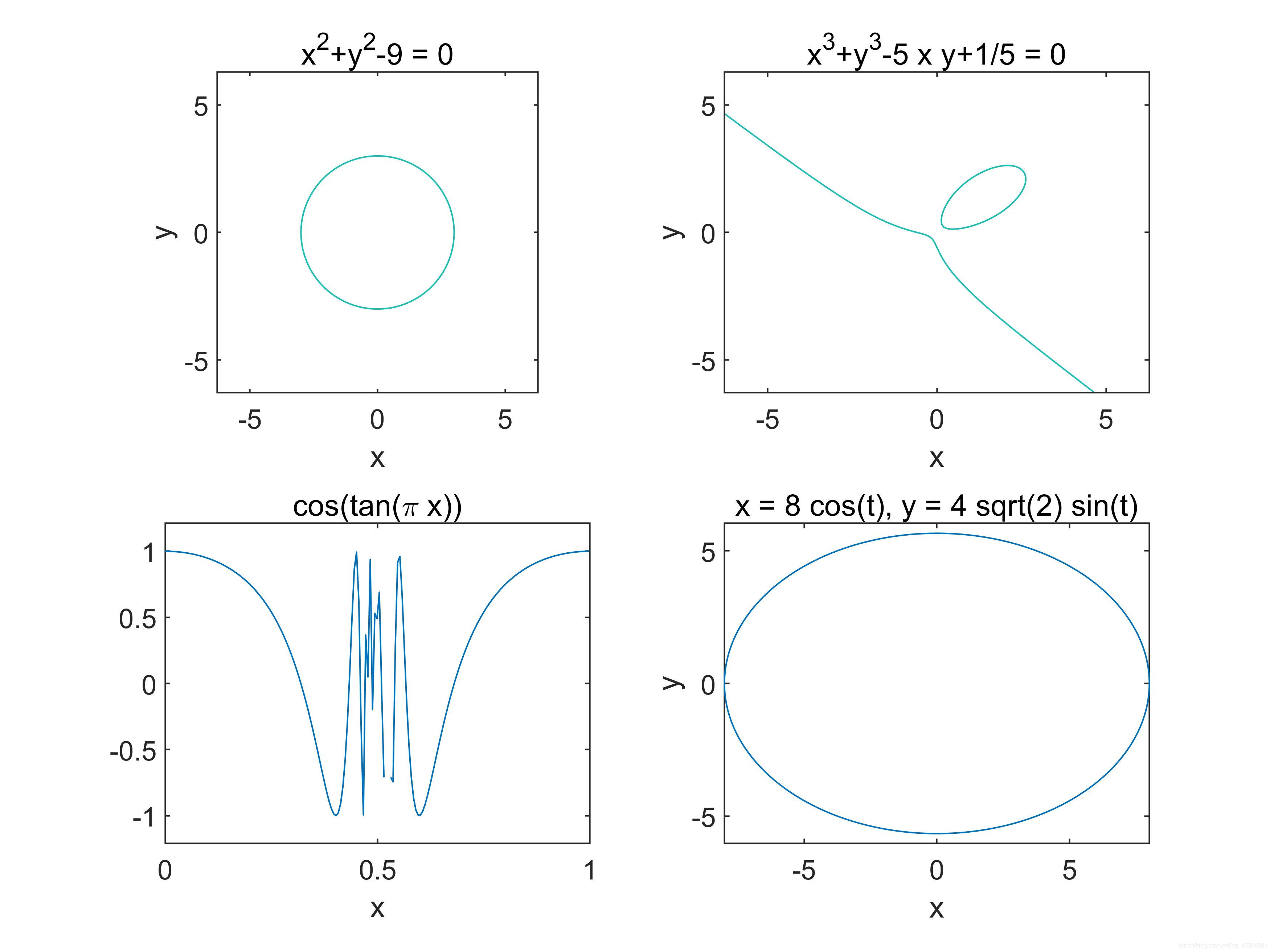
❤隐函数作图
Matlab提供了ezplot函数绘制隐函数图形,用法如下:
①对于函数f=f(x),ezplot的调用格式为:
ezplot(f); %在默认区间(-2pi,2pi)绘制图形
ezplot(f,[a,b]); %在区间(a,b)绘制图形
②对于隐函数f=f(x,y),ezplot的调用格式为:
ezplot(f); %在默认区间(-2pi,2pi)绘制f(x,y)=0的图形
ezplot(f,[xmin,xmax,ymin,ymax]); %在区间[xmin,xmax,ymin,ymax]绘制图形
ezplot(f,[a,b]); %在区间(a,b)绘制图形
③对于参数方程x=x(t),y=y(t),ezplot函数的调用格式为:
ezplot(x,y); %在默认区间绘制x=x(t),y=y(t)图形
ezplot(x,y,[tmin,tmax]); %在区间(tmin,tmax)绘制x=x(t),y=y(t)图形
其他隐函数绘图还有ezpolar,ezcontour,ezplot3,ezmesh,ezmeshc,ezsurf,ezsurfc。
例子:
subplot(2,2,1);
ezplot('x^2+y^2-9');axis equal;
subplot(2,2,2);
ezplot('x^3+y^3-5*x*y+1/5')
subplot(2,2,3);
ezplot('cos(tan(pi*x))',[0,1]);
subplot(2,2,4);
ezplot('8*cos(t)','4*sqrt(2)*sin(t)',[0,2*pi]);
版权声明:本文为qq_45384561原创文章,遵循CC 4.0 BY-SA版权协议,转载请附上原文出处链接和本声明。