机器学习--线性回归之PM2.5的预测

一、报告要求说明

采用北京大学搜集的2013-2017年的各个地区每日每小时空气品质数据
数据选用：空气品质指标(自选其一)
PM2.5、TEMP等
当日数值(自选其一)
平均值、12:00等
参数选用
前N天预测当天数据
3<=N<=20
Training Set
自行选择北京某一地区某一年度的数据
Test Set(自选其一)
同地区不同年度或者同年度不同地区
Learing rate自行设定(设定个数>3)
在学习过程中记录每一次的Error值并且画出学习曲线
计算出不同 Learing rate 下的Training set 和Test Set 的误差
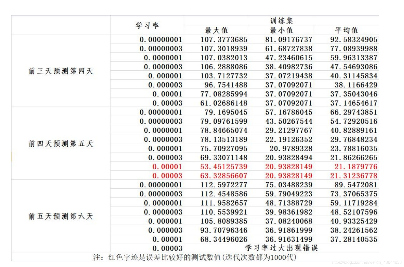
记录执行30次Training的最大误差、最小误差以及平均误差

二、数据采用

Training Set
2015 年顺义每天中午 12 点的 PM2.5 数据
Test Set
2016 年顺义每天中午 12 点的 PM2.5 数据
Learing rate（8个）
0.00000001,0.00000003,0.0000001, 0.0000003,0.000001,0.000003,0.00001, 0.00003
用前三天预测第四天
数据用excel或直接用python处理成以下格式

三、知识储备

线性回归模型来拟合数据
首先，我们将创建一个以参数θ为特征函数的代价函数:
期中：
batch gradient decent（批量梯度下降）
normal equation(正规方程法)

正规方程是通过求解下面的方程来找出使得代价函数最小的参数的：
在这里插入图片描述
假设我们的训练集特征矩阵为 X（包含了X₀=1）并且我们的训练集结果为向量 y，则利用正规方程解出向量 ,并且我们的训练集结果为向量 y，则利用正规方程解出向量：

上标T代表矩阵转置，上标-1 代表矩阵的逆。
设矩阵:
在这里插入图片描述
则:

正规方程与梯度下降函数的比较
1）梯度下降：需要选择学习率α，需要多次迭代，当特征数量n大时也能较好适用，适用于各种类型的模型
2）正规方程：不需要选择学习率α，一次计算得出，需要计算：

如果特征数量n较大则运算代价大，因为矩阵逆的计算时间复杂度为O(n3)，通常来说当n小于10000 时还是可以接受的，只适用于线性模型，不适合逻辑回归模型等其他模型。

四、代码的实现过程

数据整理(将数据分组)

def data_collation(data,day):
    x=[]
    #将数据一共分为len(data)//day组，x为前day天的数据,y为标记验证的数据
    for i in range(0,len(data)//day,day):
            mat=data.values[i:i+day,2]
            x.append(mat)
    x1=np.array(x)
    cols=x1.shape[1]
    x=x1[:,0:cols-1:]#x是所有行，去掉最后一列
    y=x1[:,cols-1:cols]#x是所有行，最后一列
    return x,y

代价函数

def computeCost(X, y, theta):
    inner = np.power(((X * theta.T) - y), 2)
    return np.sum(inner) / (2 * len(X))

batch gradient decent（批量梯度下降）

def gradientDescent(X, y, theta, alpha, iters,day,train_data):
    temp = np.matrix(np.zeros(theta.shape))
    parameters = int(theta.ravel().shape[1])
    cost = np.zeros(iters)
    for i in range(iters):
        error = (X * theta.T) - y
        for j in range(parameters):
            term = np.multiply(error, X[:, j])
            temp[0, j] = theta[0, j] - ((alpha / len(X)) * np.sum(term))
        theta = temp
        cost[i] = (computeCost(X, y, theta))/(len(train_data)/day)
    return theta, cost

normal equation(正规方程法)

def normalEqn(X, y):
    theta = np.linalg.inv(X.T@X)@X.T@y#X.T@X等价于X.T.dot(X)
    return theta

注：正规函数和梯度下降函数计算出来的值会有一些差别调整如下：

	final_theta2 = normalEqn(x_train, y_train)  # 感觉和批量梯度下降的theta的值有点差距
    #矩阵转置
    final_theta2=np.mat(final_theta2)
    final_theta2=final_theta2.T

误差可视化

def show_cost(cost,alpha):
    cost = np.array(cost)
    for i in range(0,len(cost)):
        plt.plot(cost[i],label=alpha[i])
    plt.legend(loc=1)
    plt.xlabel("迭代次数",fontsize=14)
    plt.ylabel("误差",fontsize=14)
    plt.title("误差与训练状态",fontsize=14)
    plt.show()

五、执行结果

前三天预测第四天，迭代次数1000代：
1）学习曲线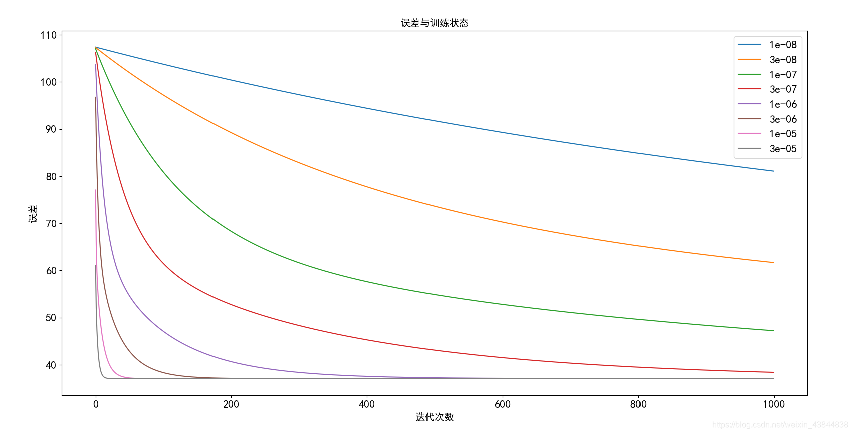

2）误差值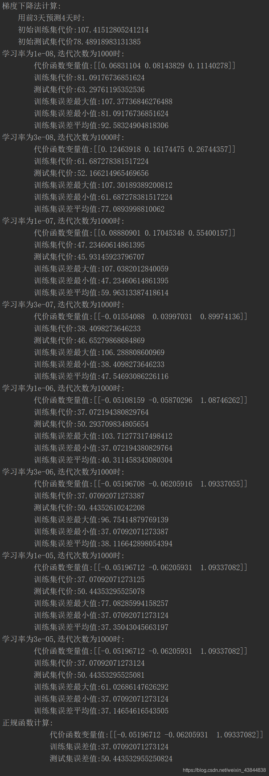
前三天预测第四天，迭代次数10000代：
1）学习曲线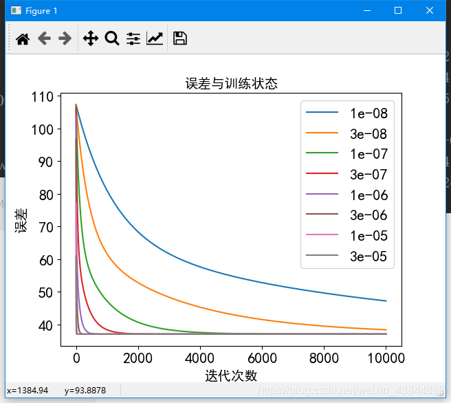

2）误差值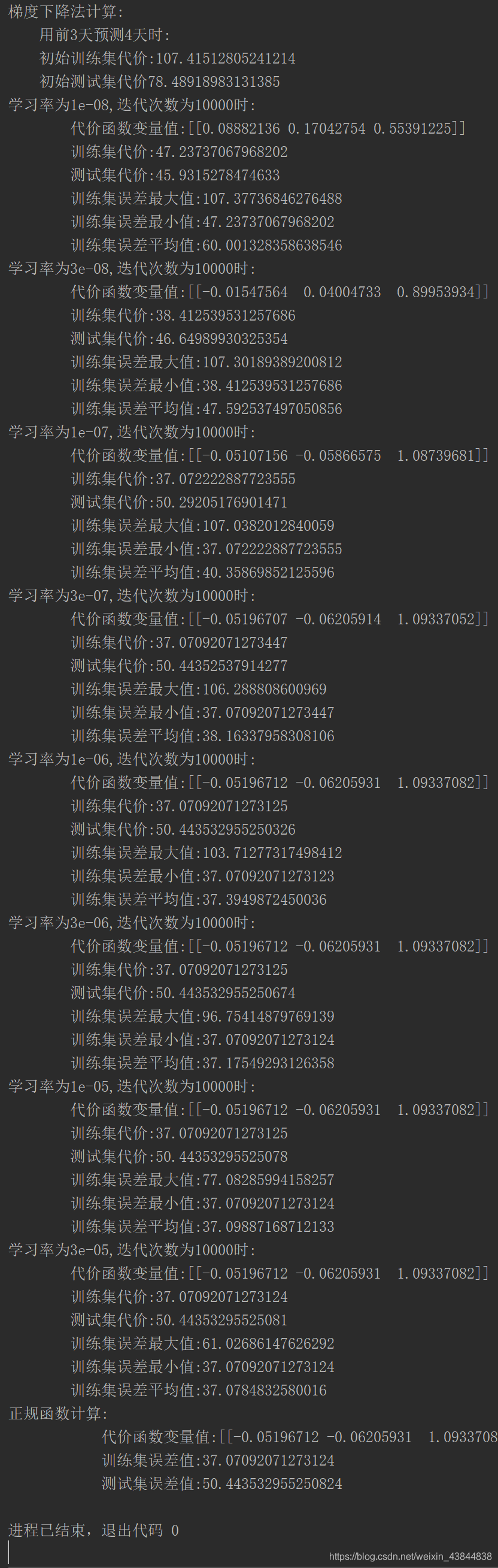
前三天预测第四天，迭代次数100000代：
1)学习曲线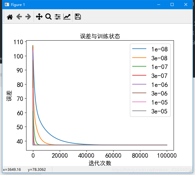

2)误差值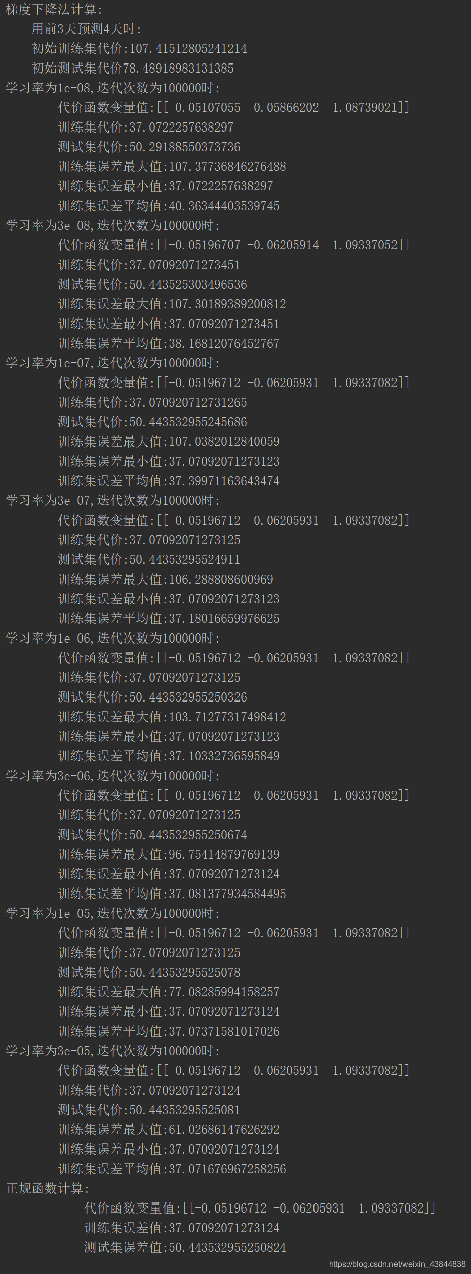
Training误差的最大值、最小值与平均值

六、完整代码

#线性回归模型
import pandas as pd
import numpy as np
import matplotlib.pyplot as plt
# 设置字体的更多属性
font = {
    'family': 'SimHei',
    'weight': 'bold',
    'size': '16'
}
plt.rc('font', **font)
# 解决坐标轴负轴的符号显示的问题
plt.rc('axes', unicode_minus=False)
#显示初始的PM2.5分布
def train_data_plt(train_data):
    #用Plt显示数据文件的分布
    plt.title("训练集分布",fontsize=20)
    plt.scatter(train_data["date"],train_data["PM2.5"],marker='o',label="PM2.5")
    plt.xlabel("year",fontsize=14)
    plt.ylabel("PM2.5",fontsize=14)
    plt.legend(loc=1)
    plt.show()
#创建一个代价函数
def computeCost(X, y, theta):
    inner = np.power(((X * theta.T) - y), 2)
    return np.sum(inner) / (2 * len(X))
#创建一个批量梯度下降的函数
def gradientDescent(X, y, theta, alpha, iters,day,train_data):
    temp = np.matrix(np.zeros(theta.shape))
    parameters = int(theta.ravel().shape[1])
    cost = np.zeros(iters)
    for i in range(iters):
        error = (X * theta.T) - y
        for j in range(parameters):
            term = np.multiply(error, X[:, j])
            temp[0, j] = theta[0, j] - ((alpha / len(X)) * np.sum(term))
        theta = temp
        cost[i] = (computeCost(X, y, theta))/(len(train_data)/day)
    return theta, cost
#数据的整理
def data_collation(data,day):
    x=[]
    for i in range(0,len(data)//day,day):
            mat=data.values[i:i+day,2]
            x.append(mat)
    x1=np.array(x)
    # print(f"x1:{x1}")
    cols=x1.shape[1]
    x=x1[:,0:cols-1:]#x是所有行，去掉最后一列
    y=x1[:,cols-1:cols]#x是所有行，最后一列
    return x,y
#有随机梯度下降函数优化过程中出现的误差值(可视化)
def show_cost(cost,alpha):
    cost = np.array(cost)
    for i in range(0,len(cost)):
        plt.plot(cost[i],label=alpha[i])
    plt.legend(loc=1)
    plt.xlabel("迭代次数",fontsize=14)
    plt.ylabel("误差",fontsize=14)
    plt.title("误差与训练状态",fontsize=14)
    plt.show()
#计算误差过程以及误差之间的处理
def cost_data(x_train, y_train, theta,alpha,iters, day, train_data):
    cost=[]
    g=[]
    for i in range(len(alpha)):
        g_c, cost_c = gradientDescent(x_train, y_train, theta, alpha[i], iters, day, train_data)
        cost.append(cost_c)
        g.append(g_c)
    g = np.array(g)
    return g,cost
#正规函数
def normalEqn(X, y):
    theta = np.linalg.inv(X.T@X)@X.T@y#X.T@X等价于X.T.dot(X)
    return theta
#主函数
def main():
    # 读取数据文件
    train_data = pd.read_csv("Shunyi_2015_12_pm2.5.csv", names=["date", "PM2.5"])
    test_data = pd.read_csv("Shunyi_2016_PM2_5.csv",names=["data","PM2.5"])
    train_data_plt(train_data)
    #测试天数(前三天测试第四天)
    day=4
    #训练集
    train_data.insert(0,"ones",1)
    #训练集数据整理
    x_train,y_train=data_collation(train_data,day)
    x_train=np.matrix(x_train)
    y_train=np.matrix(y_train)
    # 测试集
    test_data.insert(0,"ones",1)
    #测试集数据整理
    x_test,y_test=data_collation(test_data,day)
    x_test,y_test = np.matrix(x_test),np.matrix(y_test)
    print(len(train_data))
    theta = np.matrix(np.array(np.zeros(day-1)))
    # 初始代价函数
    computeCost(x_train, y_train, theta)
    print(f"梯度下降法计算:\n\
    用前{day-1}天预测{day}天时:\n\
    初始训练集代价:{computeCost(x_train, y_train, theta) /(len(train_data)/day)}\n\
    初始测试集代价{computeCost(x_test, y_test, theta) /(len(test_data)/day)}")
    # 初始化学习速率和执行的迭代次数0.00000001,0.0000001,0.000001,0.000003，0.00001，0.00003
    alpha = [0.00000001,0.00000003,0.0000001,0.0000003,0.000001,0.000003,0.00001,0.00003]
    iters = 1000
    #计算误差和函数
    g_train,cost_train=cost_data(x_train, y_train, theta, alpha, iters,day,train_data)
    show_cost(cost_train,alpha)
    #测试集
    for i in range(len(alpha)):
        print(f"学习率为{alpha[i]},迭代次数为{iters}时:\n\
        代价函数变量值:{g_train[i]}\n\
        训练集代价:{computeCost(x_train, y_train, g_train[i])/(len(train_data)/day)}\n\
        测试集代价:{computeCost(x_test, y_test, g_train[i])/(len(test_data)/day)}\n\
        训练集误差最大值:{cost_train[i].max()}\n\
        训练集误差最小值:{cost_train[i].min()}\n\
        训练集误差平均值:{cost_train[i].mean()}")
    #正规函数
    final_theta2 = normalEqn(x_train, y_train)  # 感觉和批量梯度下降的theta的值有点差距
    #矩阵转置
    final_theta2=np.mat(final_theta2)
    final_theta2=final_theta2.T
    #计算代价
    computeCost(x_train, y_train, final_theta2)
    print(f"正规函数计算:\n\
            代价函数变量值:{final_theta2}\n\
            训练集误差值:{computeCost(x_train, y_train, final_theta2)/(len(train_data)/day)}\n\
            测试集误差值:{computeCost(x_test, y_test, final_theta2)/(len(test_data)/day)}")
if __name__ =="__main__":
    main()

七、准确度的提升

模型改进的方向
(1)将一年的数据提升为两年或者更多
(2)在构建模型时，应充分考虑PM2.5与其他大气成分之间的关系，构建更合理的模型。

希望能更清晰地的帮助你理解机器学习的线性回归模型，如果有不足之处请指出，欢迎多多转载，如需转载请注明出处，谢谢

原文链接：https://blog.csdn.net/weixin_43844838/article/details/104864846