0 动机

通过普通的神经网络可以实现，但是现在图片越来越大，如果通过 NN 来实现，训练的参数太多。例如 224 x 224 x 3 = 150,528，隐藏层设置为 1024 就需要训练参数 150,528 x 1024 = 1.5 亿个，这还是第一层，因此会导致我们的网络很庞大。

另一个问题就是特征位置在不同的图片中会发生变化。例如小猫的脸在不同图片中可能位于左上角或者右下角，因此小猫的脸不会激活同一个神经元。

CNN相较于全连接能够实现参数的共享。当使用一个具有9个卷积核、大小为5*5、步长为1的滤波器对一个大小为224 x 224 x 3 的图片进行卷积时，其参数量大小：(5 x 5+1) x 9 x 3 = 702
注：不同通道之间的参数不共享。

1. Conv

Conv的原理示意图：

代码：

class Conv3x3:
    # 卷积层使用3*3的filter.
    def __init__(self, num_filters):
        self.num_filters = num_filters
        self.filters = np.random.randn(num_filters, 3, 3) / 9       # 除以9是为了减小初始值的方差
        
    def iterate_regions(self, image):
        h, w = image.shape
        
        for i in range(h - 2):                                   # (h-2)/(w-2)是滤波以单位为1的步长，所需要移动的步数
            for j in range(w - 2):
                im_region = image[i:(i + 3), j:(j + 3)]          # （i+3） 3*3的filter所移动的区域
                yield im_region, i, j
                
    def forward(self, input):
        # 28x28
        self.last_input = input
        
        h, w = input.shape
        output = np.zeros((h - 2, w - 2, self.num_filters))      # 创建一个（h-2）*（w-2）的零矩阵用于填充每次滤波后的值
        
        for im_region, i, j in self.iterate_regions(input):
            output[i, j] = np.sum(im_region * self.filters, axis=(1, 2))
            
        return output                                            # 4*4的矩阵经过3*3的filter后得到一个2*2的矩阵
    
    def backprop(self, d_L_d_out, learn_rate):
        # d_L_d_out: the loss gradient for this layer's outputs
        # learn_rate: a float
        d_L_d_filters = np.zeros(self.filters.shape)
        
        for im_region, i, j in self.iterate_regions(self.last_input):
            for f in range(self.num_filters):
                # d_L_d_filters[f]: 3x3 matrix
                # d_L_d_out[i, j, f]: num
                # im_region: 3x3 matrix in image
                d_L_d_filters[f] += d_L_d_out[i, j, f] * im_region
                
        # Update filters
        self.filters -= learn_rate * d_L_d_filters
        
        # We aren't returning anything here since we use Conv3x3 as
        # the first layer in our CNN. Otherwise, we'd need to return
        # the loss gradient for this layer's inputs, just like every
        # other layer in our CNN.
        return None

2. MaxPool

MaxPool的原理示意图：

代码：

class MaxPool2:
    # A Max Pooling layer using a pool size of 2.

    def iterate_regions(self, image):
        '''
        Generates non-overlapping 2x2 image regions to pool over.
        - image is a 2d numpy array
        '''
        # image: 3d matix of conv layer
        
        h, w, _ = image.shape
        new_h = h // 2
        new_w = w // 2

        for i in range(new_h):
            for j in range(new_w):
                im_region = image[(i * 2):(i * 2 + 2), (j * 2):(j * 2 + 2)]
                yield im_region, i, j

    def forward(self, input):
        '''
        Performs a forward pass of the maxpool layer using the given input.
        Returns a 3d numpy array with dimensions (h / 2, w / 2, num_filters).
        - input is a 3d numpy array with dimensions (h, w, num_filters)
        '''
        # 26x26x8
        self.last_input = input
        
        # input: 3d matrix of conv layer
        h, w, num_filters = input.shape
        output = np.zeros((h // 2, w // 2, num_filters))

        for im_region, i, j in self.iterate_regions(input):
            output[i, j] = np.amax(im_region, axis=(0, 1))
        
        return output
        
    def backprop(self, d_L_d_out):
        # d_L_d_out: the loss gradient for the layer's outputs
        
        d_L_d_input = np.zeros(self.last_input.shape)
        
        for im_region, i, j in self.iterate_regions(self.last_input):
            h, w, f = im_region.shape
            amax = np.amax(im_region, axis=(0, 1))
            
            for i2 in range(h):
                for j2 in range(w):
                    for f2 in range(f):
                        # If this pixel was the max value, copy the gradient to it.
                        if im_region[i2, j2, f2] == amax[f2]:
                            d_L_d_input[i + i2, j + j2, f2] = d_L_d_out[i, j, f2]
                            
        return d_L_d_input

3. Softmax

Softmax的用法：
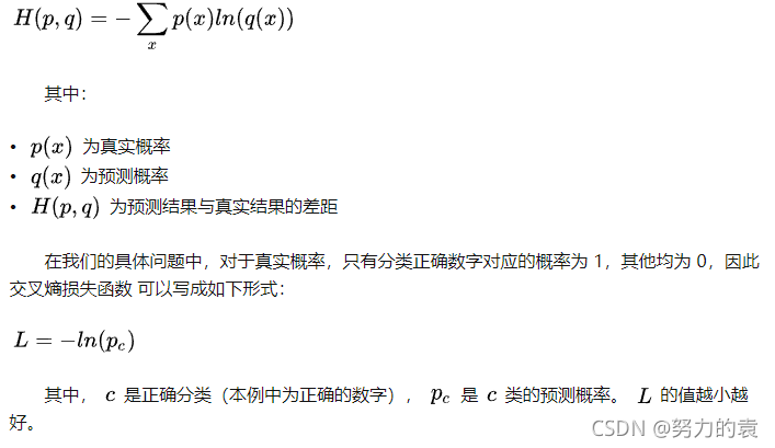
使用一个含有 10 个节点（分别代表相应数字）的 softmax 层，作为 CNN 的最后一层。最后一层为一个全连接层，只是激活函数为 softmax。经过 softmax 的变换，数字就是具有最高概率的节点。
交叉熵损失函数（Cross-Entropy Loss）：

代码：

class Softmax:
    # A standard fully-connected layer with softmax activation.
    
    def __init__(self, input_len, nodes):
        # We divide by input_len to reduce the variance of our initial values
        # input_len: length of input nodes
        # nodes: lenght of ouput nodes
        
        self.weights = np.random.randn(input_len, nodes) / input_len
        self.biases = np.zeros(nodes)

    def forward(self, input):
        '''
        Performs a forward pass of the softmax layer using the given input.
        Returns a 1d numpy array containing the respective probability values.
        - input can be any array with any dimensions.
        '''
        # 3d
        self.last_input_shape = input.shape
        
        # 3d to 1d
        input = input.flatten()
        
        # 1d vector after flatting
        self.last_input = input

        input_len, nodes = self.weights.shape

        totals = np.dot(input, self.weights) + self.biases
        
        # output before softmax
        # 1d vector
        self.last_totals = totals
        
        exp = np.exp(totals)
        return exp / np.sum(exp, axis=0)
    
    def backprop(self, d_L_d_out, learn_rate):
        # only 1 element of d_L_d_out is nonzero
        for i, gradient in enumerate(d_L_d_out):
            # k != c, gradient = 0
            # k == c, gradient = 1
            # try to find i when k == c
            if gradient == 0:
                continue
        
            # e^totals
            t_exp = np.exp(self.last_totals)
        
            # Sum of all e^totals
            S = np.sum(t_exp)
            
            # Gradients of out[i] against totals
            # all gradients are given value with k != c
            d_out_d_t = -t_exp[i] * t_exp / (S ** 2)
            # change the value of k == c
            d_out_d_t[i] = t_exp[i] * (S - t_exp[i]) / (S ** 2)
        
            # Gradients of out[i] against totals
            # gradients to every weight in every node
            # this is not the final results
            d_t_d_w = self.last_input  # vector
            d_t_d_b = 1
            # 1000 x 10
            d_t_d_inputs = self.weights
        
            # Gradients of loss against totals
            # d_L_d_t, d_out_d_t, vector, 10 elements
            d_L_d_t = gradient * d_out_d_t
        
            # Gradients of loss against weights/biases/input
            # (1000, 1) @ (1, 10) to (1000, 10)
            d_L_d_w = d_t_d_w[np.newaxis].T @ d_L_d_t[np.newaxis]
            d_L_d_b = d_L_d_t * d_t_d_b
            # (1000, 10) @ (10, 1)
            d_L_d_inputs = d_t_d_inputs @ d_L_d_t
        
            # Update weights / biases
            self.weights -= learn_rate * d_L_d_w
            self.biases -= learn_rate * d_L_d_b
        
            # it will be used in previous pooling layer
            # reshape into that matrix
            return d_L_d_inputs.reshape(self.last_input_shape)
            
# We only use the first 1k testing examples (out of 10k total)
# in the interest of time. Feel free to change this if you want.
test_images = mnist.test_images()[:1000]
test_labels = mnist.test_labels()[:1000]

# We only use the first 1k examples of each set in the interest of time.
# Feel free to change this if you want.
train_images = mnist.train_images()[:1000]
train_labels = mnist.train_labels()[:1000]
test_images = mnist.test_images()[:1000]
test_labels = mnist.test_labels()[:1000]

conv = Conv3x3(8)                    # 28x28x1 -> 26x26x8
pool = MaxPool2()                    # 26x26x8 -> 13x13x8
softmax = Softmax(13 * 13 * 8, 10)    # 13x13x8 -> 10

def forward(image, label):
    '''
    Completes a forward pass of the CNN and calculates the accuracy and
    cross-entropy loss.
    - image is a 2d numpy array
    - label is a digit
    '''
    # We transform the image from [0, 255] to [-0.5, 0.5] to make it easier
    # to work with. This is standard practice.
    out = conv.forward((image / 255) - 0.5)
    out = pool.forward(out)
    out = softmax.forward(out)

    # Calculate cross-entropy loss and accuracy. np.log() is the natural log.
    loss = -np.log(out[label])
    acc = 1 if np.argmax(out) == label else 0

    return out, loss, acc
    
    # out: vertor of probability
    # loss: num
    # acc: 1 or 0

4. Train

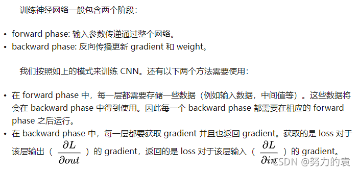
训练概述：

代码:

def train(im, label, lr=0.01):
    # Forward
    out, loss, acc = forward(im, label)
    
    # Calculate intial gradient
    gradient = np.zeros(10)
    gradient[label] = -1 / out[label]
    
    # Backprop
    gradient = softmax.backprop(gradient, lr)
    gradient = pool.backprop(gradient)
    gradient = conv.backprop(gradient, lr)
    
    return loss, acc
    
print('MNIST CNN initialized!')


# Train the CNN for 3 epochs
for epoch in range(50):
    print('--- Epoch %d ---' % (epoch + 1))
    
    # Shuffle the training data
    permutation = np.random.permutation(len(train_images))
    train_images = train_images[permutation]
    train_labels = train_labels[permutation]
    
    # Train
    loss = 0
    num_correct = 0
    # i: index
    # im: image
    # label: label
    for i, (im, label) in enumerate(zip(train_images, train_labels)):
        if i > 0 and i % 100 == 99:
            print(
                '[Step %d] Past 100 steps: Average Loss %.3f | Accuracy: %d%%' %
                (i + 1, loss / 100, num_correct)
            )
            loss = 0
            num_correct = 0

        l, acc = train(im, label)
        loss += 1
        num_correct += acc
        
# Test the CNN
print('\n--- Testing the CNN ---')
loss = 0
num_correct = 0
for im, label in zip(test_images, test_labels):
    _, l, acc = forward(im, label)
    loss += l
    num_correct += acc

num_tests = len(test_images)
print('Test Loss:', loss / num_tests)
print('Test Accuracy:', num_correct / num_tests)

结果：

MNIST CNN initialized!
--- Epoch 1 ---
[Step 100] Past 100 steps: Average Loss 0.990 | Accuracy: 17%
[Step 200] Past 100 steps: Average Loss 1.000 | Accuracy: 30%
[Step 300] Past 100 steps: Average Loss 1.000 | Accuracy: 39%
[Step 400] Past 100 steps: Average Loss 1.000 | Accuracy: 62%
[Step 500] Past 100 steps: Average Loss 1.000 | Accuracy: 67%
[Step 600] Past 100 steps: Average Loss 1.000 | Accuracy: 64%
[Step 700] Past 100 steps: Average Loss 1.000 | Accuracy: 72%
[Step 800] Past 100 steps: Average Loss 1.000 | Accuracy: 72%
[Step 900] Past 100 steps: Average Loss 1.000 | Accuracy: 80%
[Step 1000] Past 100 steps: Average Loss 1.000 | Accuracy: 77%
--- Epoch 2 ---
[Step 100] Past 100 steps: Average Loss 0.990 | Accuracy: 84%
[Step 200] Past 100 steps: Average Loss 1.000 | Accuracy: 76%
[Step 300] Past 100 steps: Average Loss 1.000 | Accuracy: 81%
[Step 400] Past 100 steps: Average Loss 1.000 | Accuracy: 78%
[Step 500] Past 100 steps: Average Loss 1.000 | Accuracy: 85%
[Step 600] Past 100 steps: Average Loss 1.000 | Accuracy: 86%
[Step 700] Past 100 steps: Average Loss 1.000 | Accuracy: 87%
[Step 800] Past 100 steps: Average Loss 1.000 | Accuracy: 86%
[Step 900] Past 100 steps: Average Loss 1.000 | Accuracy: 88%
[Step 1000] Past 100 steps: Average Loss 1.000 | Accuracy: 77%
--- Epoch 3 ---
[Step 100] Past 100 steps: Average Loss 0.990 | Accuracy: 90%
[Step 200] Past 100 steps: Average Loss 1.000 | Accuracy: 85%
[Step 300] Past 100 steps: Average Loss 1.000 | Accuracy: 84%
[Step 400] Past 100 steps: Average Loss 1.000 | Accuracy: 85%
[Step 500] Past 100 steps: Average Loss 1.000 | Accuracy: 86%
[Step 600] Past 100 steps: Average Loss 1.000 | Accuracy: 86%
[Step 700] Past 100 steps: Average Loss 1.000 | Accuracy: 91%
[Step 800] Past 100 steps: Average Loss 1.000 | Accuracy: 83%
[Step 900] Past 100 steps: Average Loss 1.000 | Accuracy: 81%
[Step 1000] Past 100 steps: Average Loss 1.000 | Accuracy: 82%

--- Testing the CNN ---
Test Loss: 0.5717330897439417
Test Accuracy: 0.817

原文链接：https://blog.csdn.net/qq_44747572/article/details/120949318