参考文章：
RNA-seq(7): DEseq2筛选差异表达基因并注释
转录组入门7-用DESeq2进行差异表达分析
Analyzing RNA-seq data with DESeq2
RNA-seq练习 第三部分（DEseq2筛选差异表达基因,可视化）

1.关于DESeq2的概述

A basic task in the analysis of count data from RNA-seq is the detection of differentially expressed genes. The count data are presented as a table which reports, for each sample, the number of sequence fragments that have been assigned to each gene. Analogous data also arise for other assay types, including comparative ChIP-Seq, HiC, shRNA screening, and mass spectrometry. An important analysis question is the quantification and statistical inference of systematic changes between conditions, as compared to within-condition variability. The package DESeq2 provides methods to test for differential expression by use of negative binomial generalized linear models; the estimates of dispersion and logarithmic fold changes incorporate data-driven prior distributions.

2.DESeq2包的安装

#对于R3.6以上版本，首先安装BiocManager软件，然后安装DESeq2软件
>BiocManager::install("DESeq2")
#依赖包会同时安装
#检查软件是否安装成功，加载
>library(DESeq2)

3.需要输入的数据结构

• count matrix（表达矩阵）—countData：就是我们前面通过read count计算后并融合生成的矩阵，行为各个基因，列为各个样品，中间为计算reads或者fragment得到的整数。

      gene_id  control_1  control_2  sh_1_1  sh_1_2  sh_2_2  sh_2_3
0610005C13Rik          0          0       4       5       1       0
0610007P14Rik        230          0    1119    1197    1868    1439
0610009B22Rik         46          0     225     272     285     228
0610009L18Rik          3          0      12      12      16      16
0610009O20Rik        157          1     684     702     499     636
0610010B08Rik          0          0       0       0      0       0

• sample information matrix（样品信息矩阵）—colData：它的类型是一个dataframe（数据框），第一列是样品名称，第二列是样品的处理情况（对照还是处理等），即condition，condition的类型是一个factor。

                 condition
       control_1   control
       control_2   control
       sh_2_1         sh_2
       sh_2_2         sh_2
       sh_2_3         sh_2

• 差异比较矩阵—design：告诉差异分析函数是要分析哪些变量间的差异，简单说就是说明哪些是对照哪些是处理。

4.载入数据

流程代码：

#调用DESeq2包
library(DESeq2)
#设置工作目录
setwd("G:/zhaoxiujuan/Rtreatment")
#设置mycounts变量
mycounts <- read.table("G:/zhaoxiujuan/Rtreatment/raw_count_file", header = T, row.names = 1)
#显示mycounts信息
head(mycounts)
#设置样品组别、重复数
condition <- factor(c(rep("control", 2), rep("sh_2", 3)), levels = c("control","sh_2"))
#显示condition设置
condition
#设置colData值
colData <- data.frame(row.names = colnames(mycounts), condition)
#显示colData值
colData

上述代码结果显示为：

> library(DESeq2)
载入需要的程辑包：S4Vectors
载入需要的程辑包：stats4
载入需要的程辑包：BiocGenerics
载入需要的程辑包：parallel
载入程辑包：‘BiocGenerics’
The following objects are masked from ‘package:parallel’:
    clusterApply, clusterApplyLB, clusterCall, clusterEvalQ, clusterExport, clusterMap, parApply, parCapply,
    parLapply, parLapplyLB, parRapply, parSapply, parSapplyLB
The following objects are masked from ‘package:stats’:
    IQR, mad, sd, var, xtabs
The following objects are masked from ‘package:base’:
    anyDuplicated, append, as.data.frame, basename, cbind, colnames, dirname, do.call, duplicated, eval, evalq,
    Filter, Find, get, grep, grepl, intersect, is.unsorted, lapply, Map, mapply, match, mget, order, paste,
    pmax, pmax.int, pmin, pmin.int, Position, rank, rbind, Reduce, rownames, sapply, setdiff, sort, table,
    tapply, union, unique, unsplit, which, which.max, which.min
载入程辑包：‘S4Vectors’
The following object is masked from ‘package:base’:
    expand.grid
载入需要的程辑包：IRanges
载入程辑包：‘IRanges’
The following object is masked from ‘package:grDevices’:
    windows
载入需要的程辑包：GenomicRanges
载入需要的程辑包：GenomeInfoDb
载入需要的程辑包：SummarizedExperiment
载入需要的程辑包：Biobase
Welcome to Bioconductor
    Vignettes contain introductory material; view with 'browseVignettes()'. To cite Bioconductor, see
    'citation("Biobase")', and for packages 'citation("pkgname")'.
载入需要的程辑包：DelayedArray
载入需要的程辑包：matrixStats
载入程辑包：‘matrixStats’
The following objects are masked from ‘package:Biobase’:
    anyMissing, rowMedians
载入需要的程辑包：BiocParallel
载入程辑包：‘DelayedArray’
The following objects are masked from ‘package:matrixStats’:
    colMaxs, colMins, colRanges, rowMaxs, rowMins, rowRanges
The following objects are masked from ‘package:base’:
    aperm, apply, rowsum
> setwd("G:/zhaoxiujuan/Rtreatment")
> mycounts <- read.table("G:/zhaoxiujuan/Rtreatment/raw_count_file", header = T, row.names = 1)
> head(mycounts)
              control_1 control_2 sh_2_1 sh_2_2 sh_2_3
0610005C13Rik         5         0      1      1      0
0610007P14Rik      1105      1268   1701   1868   1439
0610009B22Rik       148       180    253    285    228
0610009L18Rik        20        13     26     16     16
0610009O20Rik       700       609    568    499    636
0610010B08Rik         0         0      0      0      0
> condition <- factor(c(rep("control", 2), rep("sh_2", 3)), levels = c("control","sh_2"))
> condition
[1] control control sh_2    sh_2    sh_2   
Levels: control sh_2
> colData <- data.frame(row.names = colnames(mycounts), condition)
> colData
          condition
control_1   control
control_2   control
sh_2_1         sh_2
sh_2_2         sh_2
sh_2_3         sh_2

5.构建dds矩阵（三种矩阵）

流程代码：

#在R里面用于构建公式对象，~左边为因变量，右边为自变量。
#标准流程：dds <- DESeqDataSetFromMatrix(countData = cts, colData = coldata, design= ~ batch + condition) 
#countData为表达矩阵即countdata
#colData为样品信息矩阵即coldata
#design为差异表达矩阵即批次和条件（对照、处理）等
dds <- DESeqDataSetFromMatrix(mycounts, colData, design = ~condition)

上述代码结果显示为：

> dds <- DESeqDataSetFromMatrix(mycounts, colData, design = ~condition)

6.标准化

流程代码：

#对原始dds进行normalize
dds <- DESeq(dds)
#显示dds信息
dds

上述代码结果显示为：

> dds <- DESeq(dds)
estimating size factors
estimating dispersions
gene-wise dispersion estimates
mean-dispersion relationship
final dispersion estimates
fitting model and testing
> dds
class: DESeqDataSet 
dim: 24421 5 
metadata(1): version
assays(4): counts mu H cooks
rownames(24421): 0610005C13Rik 0610007P14Rik ... Zzef1 Zzz3
rowData names(22): baseMean baseVar ... deviance maxCooks
colnames(5): control_1 control_2 sh_2_1 sh_2_2 sh_2_3
colData names(2): condition sizeFactor

7.提取DESeq2分析结果

此部分使用R中排序order函数，参考：数据排序函数、R中排序函数总结

流程代码：

#使用DESeq2包中的results()函数，提取差异分析的结果
#Usage:results(object, contrast, name, .....）
#将提取的差异分析结果定义为变量"res" 
#contrast: 定义谁和谁比较
res = results(dds, contrast=c("condition", "control", "sh_2"))
#对结果res利用order()函数按pvalue值进行排序
#创建矩阵时，X[i,]指矩阵X中的第i行，X[,j]指矩阵X中的第j列
#order()函数先对数值排序，然后返回排序后各数值的索引，常用用法：V[order(V)]或者df[order(df$variable),]
res = res[order(res$pvalue),]
#显示res结果首信息
head(res)
#对res矩阵进行总结，利用summary命令统计显示一共多少个genes上调和下调
summary(res)
#将分析的所有结果进行输出保存
write.csv(res, file="All_results.csv")
#显示显著差异的数目
table(res$padj<0.05)

上述代码结果显示为：

> res = results(dds, contrast=c("condition", "control", "sh_2"))
> res = res[order(res$pvalue),]
> head(res)
log2 fold change (MLE): condition control vs sh_2 
Wald test p-value: condition control vs sh_2 
DataFrame with 6 rows and 6 columns
                baseMean    log2FoldChange             lfcSE              stat               pvalue
               <numeric>         <numeric>         <numeric>         <numeric>            <numeric>
Hhatl   436.554706238034 -3.15640255527971 0.266955557029147 -11.8237005080778 2.94423574515867e-32
Trdmt1  370.370716982041 -2.38291991440092 0.218182759967047  -10.921669130782 9.08113831015029e-28
Kcnj13  402.122939390945 -2.49666619197326 0.242026117188394 -10.3156891536208 5.98503701472684e-25
Apobec2 261.932438663556 -2.69841811678462 0.275038256583793 -9.81106465079165 1.00898329266042e-22
Fbxo2    200.42915235742 -2.56869215615048 0.270408444282014 -9.49930451680551 2.11296749482473e-21
Mgll    1339.67856033936 -1.73011450373635 0.188428278434467 -9.18181983145412 4.23866573291394e-20
                        padj
                   <numeric>
Hhatl   3.48833051086399e-28
Trdmt1  5.37966633493303e-24
Kcnj13  2.36369061834945e-21
Apobec2 2.98860851286016e-19
Fbxo2   5.00688777573669e-18
Mgll     8.3699519339274e-17
> summary(res)
out of 15686 with nonzero total read count
adjusted p-value < 0.1
LFC > 0 (up)       : 645, 4.1%
LFC < 0 (down)     : 504, 3.2%
outliers [1]       : 0, 0%
low counts [2]     : 3838, 24%
(mean count < 8)
[1] see 'cooksCutoff' argument of ?results
[2] see 'independentFiltering' argument of ?results
> write.csv(res, file="All_results.csv")
> table(res$padj<0.05)
FALSE  TRUE 
11106   742 

结果显示，一共645个基因上调，504个基因下调，没有离群值。padj小于0.05的共有742个。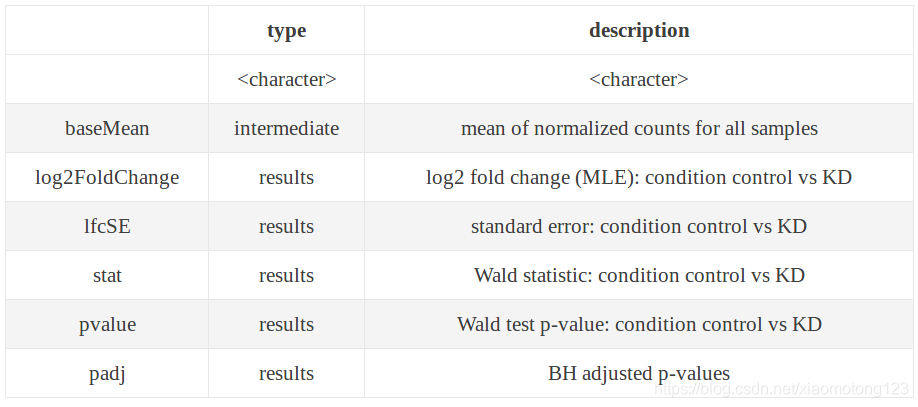

8.对具有显著性差异的结果进行提取、保存

差异表达基因的界定很不统一，但log2FC是用的最广泛同时也是最不精确的方式，但因为其好理解所以广泛被应用尤其芯片数据处理中。既然挑选差异表达基因，还是采取log2FC和padj来进行。
在利用数据比较分析两个样品中同一个基因是否存在差异表达的时候，一般选取Foldchange值和经过FDR矫正过后的p值，取padj值(p值经过多重校验校正后的值)小于0.05，log2FoldChange大于1的基因作为差异基因集。

获取padj（p值经过多重校验校正后的值）小于0.05，表达倍数取以2为对数后大于1或者小于-1的差异表达基因。

流程代码：

#使用subset()函数过滤需要的结果至新的变量diff_gene_Group2中
#Usage:subset(x, ...)，其中x为objects，...为筛选参数或条件
diff_gene_Group2 <- subset(res, padj < 0.05 & abs(log2FoldChange) > 1)
#也可以将差异倍数分开来写：
#> diff_gene_Group2 <-subset(res,padj < 0.05 & (log2FoldChange > 1 | log2FoldChange < -1))
#使用dim函数查看该结果的维度、规模
dim(diff_gene_Group2)
#显示结果的首信息
head(diff_gene_Group2)
#将结果进行输出保存
write.csv(diff_gene_Group2, file = "G:/zhaoxiujuan/Rtreatment/different_gene/different_gene_Group2_1")

上述代码结果显示为：

> diff_gene_Group2 <- subset(res, padj < 0.05 & abs(log2FoldChange) > 1)
> dim(diff_gene_Group2)
[1] 266   6
> head(diff_gene_Group2)
log2 fold change (MLE): condition sh 2 vs control 
Wald test p-value: condition sh 2 vs control 
DataFrame with 6 rows and 6 columns
                baseMean   log2FoldChange             lfcSE             stat               pvalue
               <numeric>        <numeric>         <numeric>        <numeric>            <numeric>
Hhatl   436.554706238034 3.15640255527971 0.266955557029147 11.8237005080778 2.94423574515867e-32
Trdmt1  370.370716982041 2.38291991440092 0.218182759967047  10.921669130782 9.08113831015029e-28
Kcnj13  402.122939390945 2.49666619197326 0.242026117188394 10.3156891536208 5.98503701472684e-25
Apobec2 261.932438663556 2.69841811678462 0.275038256583793 9.81106465079165 1.00898329266042e-22
Fbxo2    200.42915235742 2.56869215615048 0.270408444282014 9.49930451680551 2.11296749482473e-21
Mgll    1339.67856033936 1.73011450373635 0.188428278434467 9.18181983145412 4.23866573291394e-20
                        padj
                   <numeric>
Hhatl   3.48833051086399e-28
Trdmt1  5.37966633493303e-24
Kcnj13  2.36369061834945e-21
Apobec2 2.98860851286016e-19
Fbxo2   5.00688777573669e-18
Mgll     8.3699519339274e-17
> write.csv(diff_gene_Group2, file = "G:/zhaoxiujuan/Rtreatment/different_gene/different_gene_Group2_1")