聚类算法-分层聚类 (Clustering Algorithms - Hierarchical Clustering)
层次聚类简介 (Introduction to Hierarchical Clustering)
Hierarchical clustering is another unsupervised learning algorithm that is used to group together the unlabeled data points having similar characteristics. Hierarchical clustering algorithms falls into following two categories −
分层聚类是另一种无监督的学习算法,用于将具有相似特征的未标记数据点分组在一起。 分层聚类算法分为以下两类-
Agglomerative hierarchical algorithms − In agglomerative hierarchical algorithms, each data point is treated as a single cluster and then successively merge or agglomerate (bottom-up approach) the pairs of clusters. The hierarchy of the clusters is represented as a dendrogram or tree structure.
聚集层次算法 -在聚集层次算法中,每个数据点都被视为单个群集,然后连续合并或聚集(自下而上)群集对。 群集的层次结构表示为树状图或树结构。
Divisive hierarchical algorithms − On the other hand, in divisive hierarchical algorithms, all the data points are treated as one big cluster and the process of clustering involves dividing (Top-down approach) the one big cluster into various small clusters.
分开的分层算法 -另一方面,在分开的分层算法中,所有数据点都被视为一个大群集,并且群集过程涉及将(一个自上而下的方法)将一个大群集划分为各种小群集。
执行聚集层次聚类的步骤 (Steps to Perform Agglomerative Hierarchical Clustering)
We are going to explain the most used and important Hierarchical clustering i.e. agglomerative. The steps to perform the same is as follows −
我们将解释最常用和最重要的层次聚类,即聚类。 执行相同的步骤如下-
Step 1 − Treat each data point as single cluster. Hence, we will be having, say K clusters at start. The number of data points will also be K at start.
步骤1-将每个数据点视为单个群集。 因此,开始时我们将拥有K个群集。 开始时,数据点的数量也将为K。
Step 2 − Now, in this step we need to form a big cluster by joining two closet datapoints. This will result in total of K-1 clusters.
步骤2-现在,在这一步中,我们需要通过连接两个壁橱数据点来形成一个大型集群。 这将导致总共K-1个群集。
Step 3 − Now, to form more clusters we need to join two closet clusters. This will result in total of K-2 clusters.
步骤3-现在,要形成更多集群,我们需要加入两个壁橱集群。 这将导致总共有K-2个集群。
Step 4 − Now, to form one big cluster repeat the above three steps until K would become 0 i.e. no more data points left to join.
步骤4-现在,要形成一个大集群,请重复上述三个步骤,直到K变为0,即不再有要加入的数据点。
Step 5 − At last, after making one single big cluster, dendrograms will be used to divide into multiple clusters depending upon the problem.
步骤5-最后,在制作了一个大集群之后,将根据问题使用树状图将其划分为多个集群。
树状图在聚集层次聚类中的作用 (Role of Dendrograms in Agglomerative Hierarchical Clustering)
As we discussed in the last step, the role of dendrogram starts once the big cluster is formed. Dendrogram will be used to split the clusters into multiple cluster of related data points depending upon our problem. It can be understood with the help of following example −
正如我们在最后一步中讨论的那样,一旦大集群形成,树状图就开始发挥作用。 根据我们的问题,将使用树状图将群集分为相关数据点的多个群集。 通过以下示例可以理解-
例子1 (Example 1)
To understand, let us start with importing the required libraries as follows −
为了理解,让我们从导入所需的库开始,如下所示:
%matplotlib inline
import matplotlib.pyplot as plt
import numpy as np
Next, we will be plotting the datapoints we have taken for this example −
接下来,我们将绘制此示例中采用的数据点-
X = np.array([[7,8],[12,20],[17,19],[26,15],[32,37],[87,75],[73,85], [62,80],[73,60],[87,96],])
labels = range(1, 11)
plt.figure(figsize=(10, 7))
plt.subplots_adjust(bottom=0.1)
plt.scatter(X[:,0],X[:,1], label='True Position')
for label, x, y in zip(labels, X[:, 0], X[:, 1]):
   plt.annotate(label,xy=(x, y), xytext=(-3, 3),textcoords='offset points', ha='right', va='bottom')
plt.show()
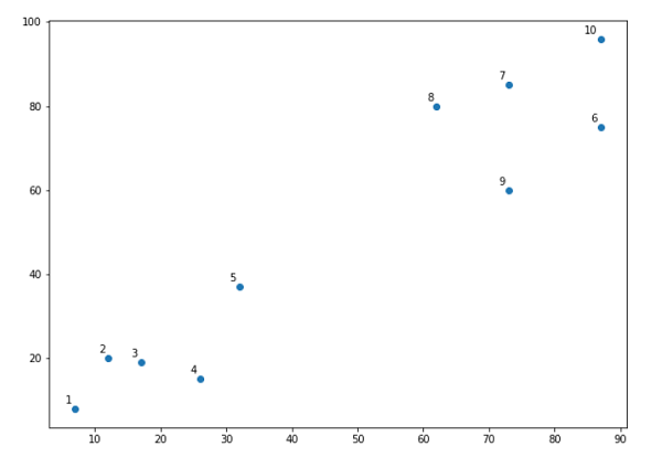
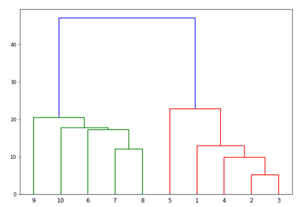
From the above diagram, it is very easy to see that we have two clusters in out datapoints but in the real world data, there can be thousands of clusters. Next, we will be plotting the dendrograms of our datapoints by using Scipy library −
从上图很容易看出,我们在数据点外有两个集群,但在现实世界的数据中,可以有成千上万个集群。 接下来,我们将使用Scipy库绘制数据点的树状图-
from scipy.cluster.hierarchy import dendrogram, linkage
from matplotlib import pyplot as plt
linked = linkage(X, 'single')
labelList = range(1, 11)
plt.figure(figsize=(10, 7))
dendrogram(linked, orientation='top',labels=labelList, distance_sort='descending',show_leaf_counts=True)
plt.show()
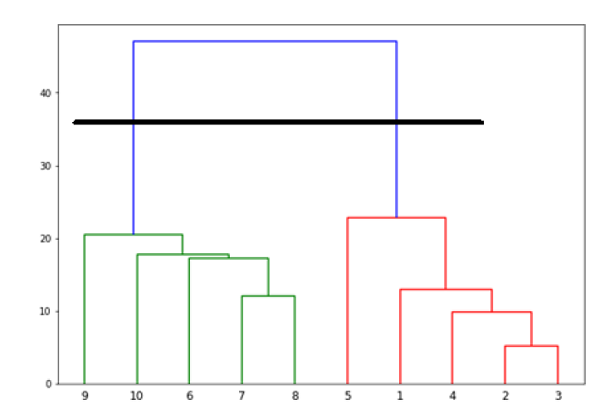
Now, once the big cluster is formed, the longest vertical distance is selected. A vertical line is then drawn through it as shown in the following diagram. As the horizontal line crosses the blue line at two points, the number of clusters would be two.
现在,一旦形成大集群,就选择了最长的垂直距离。 然后通过一条垂直线绘制一条线,如下图所示。 当水平线与蓝线在两个点处相交时,簇的数量将为两个。
Next, we need to import the class for clustering and call its fit_predict method to predict the cluster. We are importing AgglomerativeClustering class of sklearn.cluster library −
接下来,我们需要导入用于聚类的类,并调用其fit_predict方法以预测聚类。 我们正在导入sklearn.cluster库的AgglomerativeClustering类-
from sklearn.cluster import AgglomerativeClustering
cluster = AgglomerativeClustering(n_clusters=2, affinity='euclidean', linkage='ward')
cluster.fit_predict(X)
Next, plot the cluster with the help of following code −
接下来,在以下代码的帮助下绘制群集-
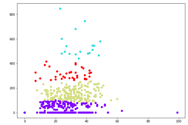
plt.scatter(X[:,0],X[:,1], c=cluster.labels_, cmap='rainbow')
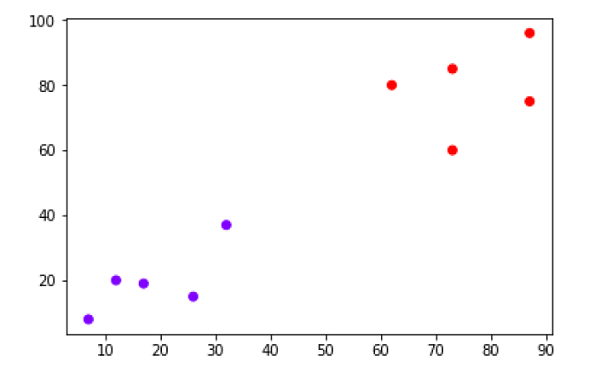
The above diagram shows the two clusters from our datapoints.
上图显示了来自我们数据点的两个群集。
例2 (Example2)
As we understood the concept of dendrograms from the simple example discussed above, let us move to another example in which we are creating clusters of the data point in Pima Indian Diabetes Dataset by using hierarchical clustering −
正如我们从上面讨论的简单示例理解树状图的概念一样,让我们转到另一个示例,在该示例中,我们将使用分层聚类在Pima Indian Diabetes Dataset中创建数据点的聚类-
import matplotlib.pyplot as plt
import pandas as pd
%matplotlib inline
import numpy as np
from pandas import read_csv
path = r"C:\pima-indians-diabetes.csv"
headernames = ['preg', 'plas', 'pres', 'skin', 'test', 'mass', 'pedi', 'age', 'class']
data = read_csv(path, names=headernames)
array = data.values
X = array[:,0:8]
Y = array[:,8]
data.shape
(768, 9)
data.head()
| slno. | preg | Plas | Pres | skin | test | mass | pedi | age | class |
|---|---|---|---|---|---|---|---|---|---|
| 0 | 6 | 148 | 72 | 35 | 0 | 33.6 | 0.627 | 50 | 1 |
| 1 | 1 | 85 | 66 | 29 | 0 | 26.6 | 0.351 | 31 | 0 |
| 2 | 8 | 183 | 64 | 0 | 0 | 23.3 | 0.672 | 32 | 1 |
| 3 | 1 | 89 | 66 | 23 | 94 | 28.1 | 0.167 | 21 | 0 |
| 4 | 0 | 137 | 40 | 35 | 168 | 43.1 | 2.288 | 33 | 1 |
| slno。 | 预浸料 | 普拉斯 | 压力 | 皮肤 | 测试 | 大众 | 佩迪 | 年龄 | 类 |
|---|---|---|---|---|---|---|---|---|---|
| 0 | 6 | 148 | 72 | 35 | 0 | 33.6 | 0.627 | 50 | 1个 |
| 1个 | 1个 | 85 | 66 | 29 | 0 | 26.6 | 0.351 | 31 | 0 |
| 2 | 8 | 183 | 64 | 0 | 0 | 23.3 | 0.672 | 32 | 1个 |
| 3 | 1个 | 89 | 66 | 23 | 94 | 28.1 | 0.167 | 21 | 0 |
| 4 | 0 | 137 | 40 | 35 | 168 | 43.1 | 2.288 | 33 | 1个 |
patient_data = data.iloc[:, 3:5].values
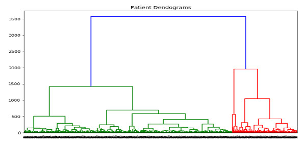
import scipy.cluster.hierarchy as shc
plt.figure(figsize=(10, 7))
plt.title("Patient Dendograms")
dend = shc.dendrogram(shc.linkage(data, method='ward'))
from sklearn.cluster import AgglomerativeClustering
cluster = AgglomerativeClustering(n_clusters=4, affinity='euclidean', linkage='ward')
cluster.fit_predict(patient_data)
plt.figure(figsize=(10, 7))
plt.scatter(patient_data[:,0], patient_data[:,1], c=cluster.labels_, cmap='rainbow')