时间序列预测 深度学习_如何使用深度学习进行时间序列预测

介绍(Introduction)

For a long time, I heard that the problem of time series could only be approached by statistical methods (AR[1], AM[2], ARMA[3], ARIMA[4]). These techniques are generally used by mathematicians who try to improve them continuously to constrain stationary and non-stationary time series.

很长时间以来，我听说只有通过统计方法(AR [1]，AM [2]，ARMA [3]，ARIMA [4])才能解决时间序列问题。 这些技术通常由数学家使用，他们试图不断对其进行改进，以约束固定和非固定的时间序列。

A friend of mine (mathematician, professor of statistics, and specialist in non-stationary time series) offered me several months ago to work on the validation and improvement of techniques to reconstruct the lightcurve of stars. Indeed, the Kepler satellite[11], like many other satellites, could not continuously measure the intensity of the luminous flux of nearby stars. The Kepler satellite was dedicated between 2009 and 2016 to search for planets outside our Solar System called extrasolar planets or exoplanets.

我的一个朋友(数学家，统计学教授，非平稳时间序列专家)几个月前邀请我来研究验证和改进重构恒星光曲线的技术。 确实，开普勒卫星[11]像许多其他卫星一样，无法连续测量附近恒星的光通量强度。 开普勒卫星专用于2009年至2016年之间，用于搜寻太阳系外的行星，称为太阳系外行星或系外行星。

As you have understood, we are going to travel a little further than our planet Earth and deep dive into a galactic journey whose machine learning will be our vessel. As you can understand, astrophysics has remained a strong passion for me.

如您所知，我们将比地球运行得更远，并深入银河之旅，其机器学习将成为我们的船只。 如您所知，天体物理学一直对我充满热情。

The notebook is available on Github: Here.

该笔记本可在Github上找到：在这里。

RNN，LSTM，GRU，双向，CNN-x (RNN, LSTM, GRU, Bidirectional, CNN-x)

So what ship will we carry through this study? We will use the recurrent neural networks (RNN[5]), models. We will use LSTM[6], GRU[7], Stacked LSTM, Stacked GRU, Bidirectional[8] LSTM, Bidirectional GRU, and also CNN-LSTM[9]. For those passionate about tree family, you can find a great article on XGBoost and time series written by Jason Brownlee here. A great repository about time series is available on github.

那么我们将进行什么样的研究呢？ 我们将使用递归神经网络(RNN [5])模型。 我们将使用LSTM [6]，GRU [7]，堆叠LSTM，堆叠GRU，双向[8] LSTM，双向GRU，以及CNN-LSTM [9]。 有关树家族的激情，你可以找到XGBoost和贾森·布朗利写了一大篇的时间序列在这里。 github上提供了有关时间序列的强大存储库。

For those who are not familiar with the RNN family, see them as learning methods with memory effect and the ability to forget. The bidirectional term comes from the architecture, it is about two RNN which will “read” the data in one direction (from left to right) and the other (from right to left) in order to be able to have the best representation of long-term dependencies.

对于那些不熟悉RNN家族的人，将它们视为具有记忆效应和忘记能力的学习方法。 双向术语来自体系结构，它是大约两个RNN，它将沿一个方向(从左到右)和另一个方向(从右到左)“读取”数据，以便能够最好地表示long项依赖项。

数据 (Data)

As said earlier in the introduction, the data correspond to flux measurements of several stars. Indeed, at each temporal increment (hour), the satellite made a measurement of the flux coming from nearby stars. This flux, or magnitude, which is light intensity, varies over time. There are several reasons for this, the proper movement of the satellite, rotation, angle of sight, etc. will vary. Therefore the number of photons measured will change, the star is a ball of molten material (hydrogen and helium fusion) which has its own movement therefore the emission of photons is made depending on its movement. This corresponds to fluctuations in light intensity.

如引言中前面所述，数据对应于几颗恒星的通量测量值。 实际上，在每个时间增量(小时)，人造卫星都对来自附近恒星的通量进行了测量。 该光通量或大小(即光强度)随时间变化。 造成这种情况的原因有很多，卫星的正确运动，旋转，视角等会有所不同。 因此，测得的光子数量将发生变化，星形是具有自身运动的熔融材料(氢和氦聚变)球，因此，光子的发射取决于其运动。 这对应于光强度的波动。

But, there can also be planets, exoplanets, which disturb the star or even pass between the star and in the line of sight of the satellite (transit method[12]). This passage obscures the star, the satellite receives fewer photons because they are blocked by the planet passing in front of it (a concrete example is a Solar eclipse due to the Moon).

但是，也可能存在行星，系外行星，它们干扰恒星，甚至在恒星之间并在卫星视线内通过(过境法[12])。 这条通道遮盖了恒星，卫星接收到的光子更少，因为它们被穿过它前面的行星所阻挡(一个具体的例子是由于月球引起的Eclipse)。

The set of flux measurements is called a light curve. What does a light curve look like? Here are some examples:

通量测量值的集合称为光曲线。 光线曲线是什么样的？ 这里有些例子：

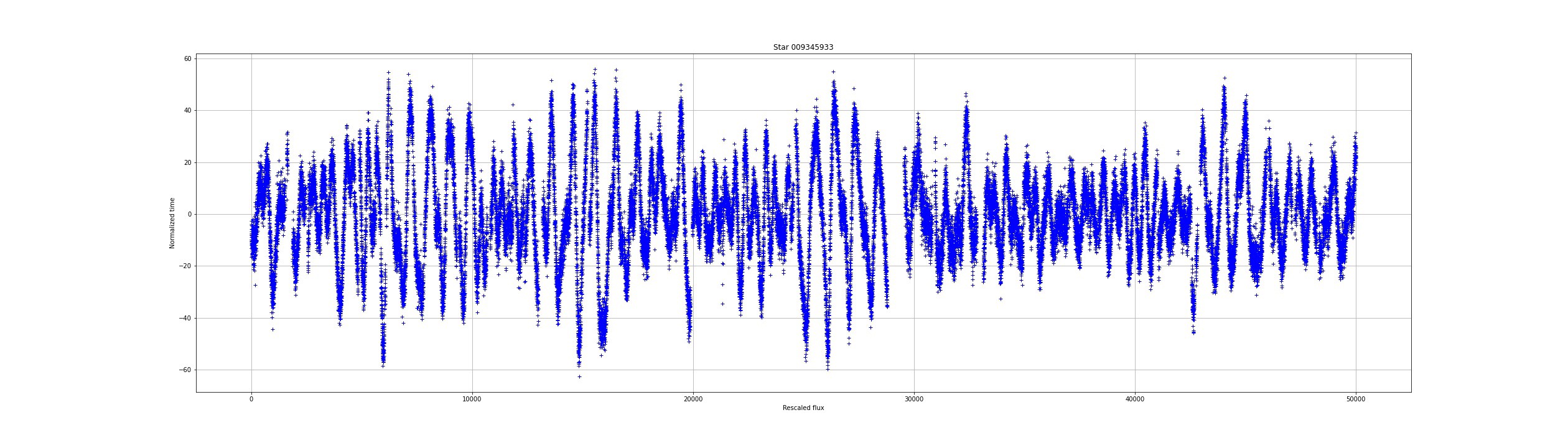
The fluxes are very different from one star to another. Some are very noisy while others have great stability. The fluxes nevertheless present anomalies. Holes, or lack of measurement, are visible in the light curves. The goal is to see if it is possible to predict the behavior of light curves where there is no measurement.

从一颗恒星到另一颗恒星的通量有很大不同。 有些嘈杂，而有些则非常稳定。 尽管如此，通量仍存在异常。 在光曲线上可以看到Kong或缺乏测量。 目的是查看是否有可能在没有测量的情况下预测光曲线的行为。

数据缩减 (Data Reduction)

In order to be able to use the data in the models, it is necessary to carry out a data reduction. Two will be presented here, the moving average and window method.

为了能够使用模型中的数据，有必要进行数据缩减。 这里将介绍两个，移动平均法和窗口法。

Moving average:

移动平均线：

The moving average consists of taking X successive points and compute the mean on them. This method permits to reduce the variability and delete the noise. This also reduces the number of points, it’s a downsampling method.

移动平均值包括获取X个连续点并计算它们的平均值。 这种方法可以减少可变性并消除噪声。 这也减少了点数，这是一种下采样方法。

The following function allows us to compute a moving average from a list of points by giving a number that will be used to compute the average and the standard deviation of the points.

下面的函数允许我们通过给出一个将用于计算点的平均值和标准偏差的数字来从点列表中计算移动平均值。

You can see that the function takes 3 parameters in the input. time and flux are the x and y of the time series. lag is the parameter controlling the number of points takes into account to compute the mean of the time and flux and the standard deviation of the flux.

您可以看到该函数在输入中带有3个参数。 时间和通量是时间序列的x和y 。 滞后是控制点数的参数，用于计算时间和通量的平均值以及通量的标准偏差。

Now, we can take a look at how to use this function and the result obtained by the transformation.

现在，我们来看看如何使用此函数以及通过转换获得的结果。

# import the packages needed for the study
matplotlib inline
import scipy
import pandas as pd
import numpy as np
import matplotlib.pyplot as plt
import sklearn
import tensorflow as tf
# let's see the progress bar
from tqdm import tqdm
tqdm().pandas()

Now we need to import the data. The file kep_lightcurves.csv contains the data from the 13 stars. Each star has 4 columns, the original flux (‘…_orig’), the rescaled flux is the original flux minus the average flux (‘…_rscl’), the difference (‘…_diff’), and the residuals (‘…_res’). So, 52 columns in total.

现在我们需要导入数据。 文件kep_lightcurves.csv包含13个星星的数据。 每颗星都有4列，原始通量(‘…_ orig’)，重新缩放的通量是原始通量减去平均通量(‘…_ rscl’)，差(‘…_ diff’)和残差(‘…_ res ‘)。 因此，总共52列。

# reduce the number of points with the mean on 20 points
x, y, y_err  = moving_mean(df.index,df["001724719_rscl"], 20)

df.index correspond to the time of the time seriesdf[“001724719_rscl”] rescaled flux of the star (“001724719”)lag=20 is the number of points where the mean and the std will be computed

df.index对应于时间序列的时间df [“ 001724719_rscl”]星的重标通量(“ 001724719”)lag = 20是将计算平均值和std的点数

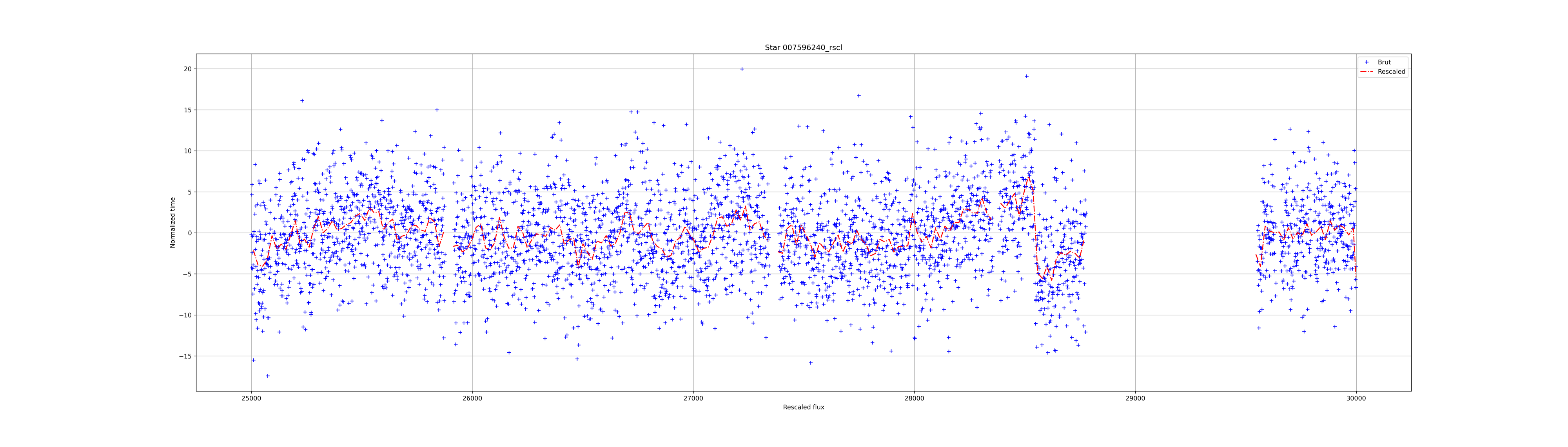
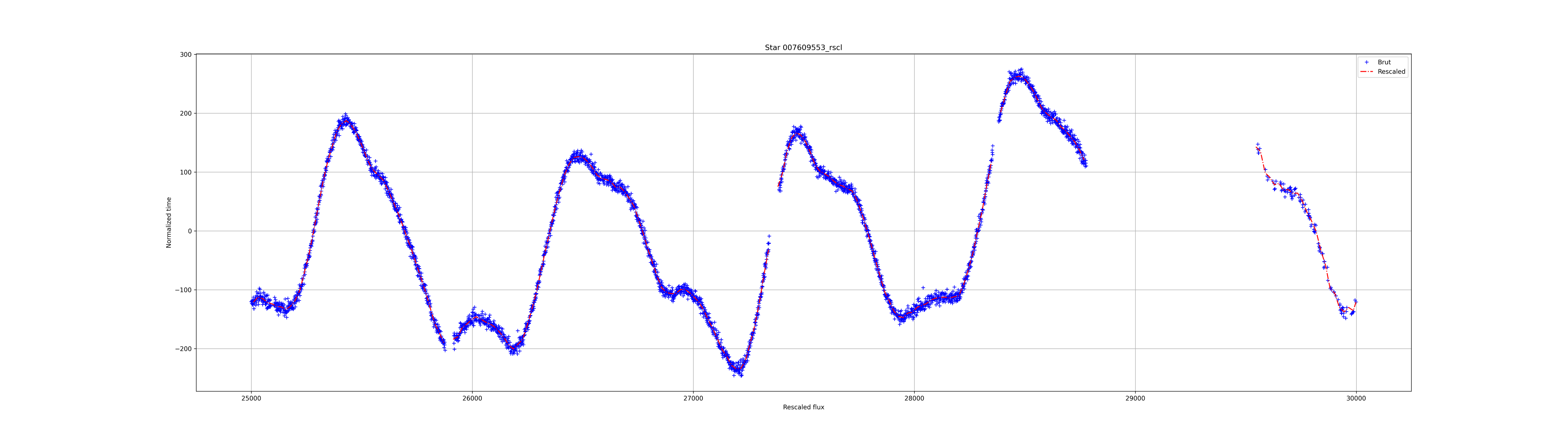
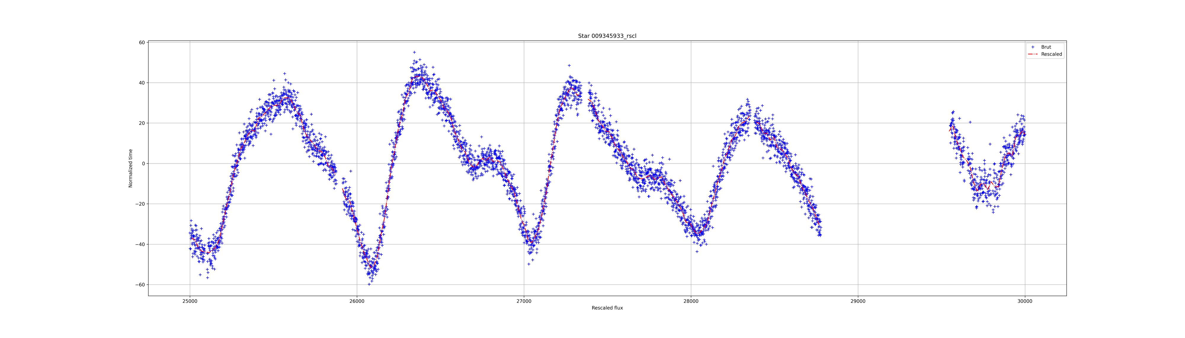
The result for the 3 previous lightcurves:

先前3个光曲线的结果：

Window Method:

窗口方法：

The second method is the window method, how does it work?

第二种方法是window方法，它如何工作？

You need to take a number of points, in the previous case 20, compute the mean (no difference with the previous method), this point it’s the beginning of the new time series and it is at the position 20 (shift of 19 points). But, instead of shifting to the next 20 points, the window is shifted by one point, compute the mean with the 20 previous points and move again and again by just shifting one step ahead. It’s not a downsampling method but a cleaning method because the effect is to smooth the data points.

您需要获取多个点，在前面的情况下为20，计算平均值(与前面的方法没有区别)，这一点是新时间序列的开始，并且在位置20(偏移19点) 。 但是，不是将窗口移动到下一个20点，而是将窗口移动了一个点，计算了前20个点的均值，并向前移动了一个步骤一次又一次地移动。 这不是缩减采样方法，而是一种清理方法，因为其效果是使数据点平滑。

Let’s see it in code:

让我们在代码中看到它：

You can easily use it like that:

您可以像这样轻松地使用它：

# reduce the number of points with the mean on 20 points
x, y, y_err  = mean_sliding_windows(df.index,df["001724719_rscl"], 40)

df.index correspond to the time of the time seriesdf[“001724719_rscl”] rescaled flux of the star (“001724719”)lag=40 is the number of points where the mean and the std will be computed

df.index对应于时间序列df[“001724719_rscl”]重新定df[“001724719_rscl”]星通量(“ 001724719”)的时间lag=40是计算均值和std的点数

Now, look at the result:

现在，看一下结果：

Well, not so bad. Setting the lag to 40 permits to “predict” or extend the new time series in the small holes. But, if you look closer you’ll see a divergence at the beginning and the end of the portions of the red line. The function can be improved to avoid these artifacts.

好吧，还不错。 将延迟设置为40可以“预测”或延长小Kong中的新时间序列。 但是，如果您仔细观察，您会在红线部分的开始和结束处看到差异。 可以改进功能以避免这些伪影。

For the rest of the study, we will use the time series obtained with the moving average method.

在其余的研究中，我们将使用通过移动平均法获得的时间序列。

Change the x-axis from values to dates:

将x轴从值更改为日期：

You can change the axis if you want with dates. The Kepler mission began on 2009–03–07 and ended in 2017. Pandas has a function called pd.data_range() this function that allows you to create dates from a list constantly incrementing.

如果需要日期，可以更改轴。 开普勒任务开始于2009-03-07在2017年结束的大熊猫有一个函数调用pd.data_range()这个函数，它允许您创建不断递增名单的日期。

df.index = pd.date_range(‘2009–03–07’, periods=len(df.index), freq=’h’)

df.index = pd.date_range('2009–03–07', periods=len(df.index), freq='h')

This line of code will create a new index with a frequency of hours. If you print the result (as below) you’ll find a proper real timescale.

这行代码将创建一个以小时为单位的新索引。 如果您打印结果(如下所示)，则会找到合适的实时刻度。

$ df.index
DatetimeIndex(['2009-03-07 00:00:00', '2009-03-07 01:00:00',
               '2009-03-07 02:00:00', '2009-03-07 03:00:00',
               '2009-03-07 04:00:00', '2009-03-07 05:00:00',
               '2009-03-07 06:00:00', '2009-03-07 07:00:00',
               '2009-03-07 08:00:00', '2009-03-07 09:00:00',
               ...
               '2017-04-29 17:00:00', '2017-04-29 18:00:00',
               '2017-04-29 19:00:00', '2017-04-29 20:00:00',
               '2017-04-29 21:00:00', '2017-04-29 22:00:00',
               '2017-04-29 23:00:00', '2017-04-30 00:00:00',
               '2017-04-30 01:00:00', '2017-04-30 02:00:00'],
              dtype='datetime64[ns]', length=71427, freq='H')

You have now a good timescale for the original time series.

现在，您对原始时间序列有了良好的时标。

Generate the datasets

生成数据集

So, now that the data reduction functions have been created, we can combine them in another function (shown below) which will take into account the initial dataset and the name of the stars present in the dataset (this part could have been done in the function).

因此，既然已经创建了数据归约函数，我们就可以将它们组合到另一个函数中(如下所示)，该函数将考虑初始数据集和数据集中存在的恒星的名称(这部分可以在功能)。

To generate the new data frames do this:

要生成新的数据帧，请执行以下操作：

stars = df.columns
stars = list(set([i.split("_")[0] for i in stars]))
print(f"The number of stars available is: {len(stars)}")
> The number of stars available is: 13

We have 13 stars with 4 data types, corresponding to 52 columns.

我们有13个恒星，具有4种数据类型，对应于52列。

df_mean, df_slide = reduced_data(df,stars)

Perfect, at this point, you have two new datasets containing the data reduced by the moving average and the window method.

完美，到此，您有了两个新的数据集，其中包含通过移动平均值和窗口法减少的数据。

方法 (Methods)

Prepare the data:

准备数据：

In order to use a machine-learning algorithm to predict time series, the data must be prepared accordingly. The data cannot just be set at (x,y) data points. The data must take the form of a series [x1, x2, x3, …, xn] and a predicted value y.

为了使用机器学习算法来预测时间序列，必须相应地准备数据。 不能仅在(x，y)数据点上设置数据。 数据必须采用序列[x1，x2，x3，…，xn]和预测值y的形式。

The function below shows you how to set up your dataset:

下面的函数向您展示如何设置数据集：

Two important things before starting.

开始之前的两个重要事项。

1- The data need to be rescaledDeep Learning algorithms are better when the data is in the range of [0, 1) to predict time series. To do it simply scikit-learn provides the function MinMaxScaler(). You can configure the feature_range parameter but by default it takes (0, 1). And clean the data of nan values (if you don’t delete the nan values your loss function will be output nan).

1-当数据在[0，1)范围内以预测时间序列时，需要重新缩放数据深度学习算法更好。 为此， scikit-learn提供了MinMaxScaler ()函数。 您可以配置feature_range参数，但默认情况下需要(0, 1) 。 并清除nan值的数据(如果不删除nan值，则损失函数将输出nan)。

# normalize the dataset 
num = 2 # choose the third star in the dataset
values = df_model[stars[num]+"_rscl_y"].values # extract the list of values
scaler = MinMaxScaler(feature_range=(0, 1)) # make an instance of MinMaxScaler
dataset = scaler.fit_transform(values[~np.isnan(values)].reshape(-1, 1)) # the data will be clean of nan values, rescaled and reshape

2- The data need to be converted into x list and y Now, we will the create_values() function to generate the data for the models. But, before, I prefer to save the original data by:

2-数据需要转换为x列表和y 现在， 我们将使用create_values()函数为模型生成数据。 但是，在此之前，我更喜欢通过以下方式保存原始数据：

df_model = df_mean.save()

df_model = df_mean.save()

# split into train and test sets
train_size = int(len(dataset) * 0.8)   # make 80% data train
train = dataset[:train_size] # set the train data
test  = dataset[train_size:] # set the test data 
# reshape into X=t and Y=t+1look_back = 20
trainX, trainY = create_dataset(train, look_back)
testX, testY = create_dataset(test, look_back)
# reshape input to be [samples, time steps, features]
trainX = np.reshape(trainX, (trainX.shape[0], trainX.shape[1], 1))
testX = np.reshape(testX, (testX.shape[0], testX.shape[1], 1))

Just take a look at the result:

看看结果：

trainX[0]
> array([[0.7414906],
       [0.76628096],
       [0.79901113],
       [0.62779976],
       [0.64012722],
       [0.64934765],
       [0.68549234],
       [0.64054092],
       [0.68075644],
       [0.73782449],
       [0.68319294],
       [0.64330245],
       [0.61339268],
       [0.62758265],
       [0.61779702],
       [0.69994317],
       [0.64737128],
       [0.64122564],
       [0.62016833],
       [0.47867125]]) # 20 values in the first value of x train datatrainY[0]
> array([0.46174275]) # the corresponding y value

Metrics

指标

What metrics do we use for time series prediction? We can use the mean absolute error and the mean squared error. They are given by the function:

我们将什么指标用于时间序列预测？ 我们可以使用平均绝对误差和均方误差。 它们由功能给出：

You need to first import the functions:

您需要首先导入功能：

from sklearn.metrics import mean_absolute_error, mean_squared_error

RNNs:

RNN：

You can implement easily the RNN family with Keras in few lines of code. Here you can use this function which will configure your RNN. You need to first import the different models from Keras like:

您可以使用几行代码轻松使用Keras实现RNN系列。 在这里，您可以使用此功能来配置您的RNN。 您需要先从Keras导入不同的模型，例如：

# import some packages
import tensorflow as tf
from keras.layers import SimpleRNN, LSTM, GRU, Bidirectional, Conv1D, MaxPooling1D, Dropout

Now, we have the models imported from Keras. The function below can generate a simple model (SimpleRNN, LSTM, GRU). Or, two models (identical) can be stacked, or used in Bidirectional or a stack of two Bidirectional models. You can also add the CNN part (Conv1D)with MaxPooling1D and dropout.

现在，我们有了从Keras导入的模型。 下面的函数可以生成一个简单的模型( SimpleRNN ， LSTM ， GRU )。 或者，两个模型(相同)可以堆叠，或在使用Bidirectional或两种双向模式的堆叠。 您还可以添加CNN部分( Conv1D含) MaxPooling1D和dropout 。

This function computes the metrics for the training part and the test part and returned the results in a data frame. Look at how you how to use it for five examples.

此函数计算训练部分和测试部分的指标，并将结果返回到数据框中。 看一下如何在五个示例中使用它。

LSTM:

LSTM：

# train the model and compute the metrics
> x_train_predict_lstm, y_train_lstm,x_test_predict_lstm, y_test_lstm, res= time_series_deep_learning(train_x, train_y, test_x, test_y, model_dl=LSTM ,  unit=12, look_back=20)
# plot the resuts of the prediction
> plotting_predictions(dataset, look_back, x_train_predict_lstm,  x_test_predict_lstm)
# save the metrics per model in the dataframe df_results
> df_results = df_results.append(res)

GRU:

GRU：

# train the model and compute the metrics
> x_train_predict_lstm, y_train_lstm,x_test_predict_lstm, y_test_lstm, res= time_series_deep_learning(train_x, train_y, test_x, test_y, model_dl=GRU,  unit=12, look_back=20)

Stack LSTM:

堆栈LSTM：

# train the model and compute the metrics
> x_train_predict_lstm, y_train_lstm,x_test_predict_lstm, y_test_lstm, res= time_series_deep_learning(train_x, train_y, test_x, test_y, model_dl=LSTM ,  unit=12, look_back=20, stacked=True)

Bidirectional LSTM:

双向LSTM：

# train the model and compute the metrics
> x_train_predict_lstm, y_train_lstm,x_test_predict_lstm, y_test_lstm, res= time_series_deep_learning(train_x, train_y, test_x, test_y, model_dl=LSTM ,  unit=12, look_back=20, bidirection=True)

CNN-LSTM:

CNN-LSTM：

# train the model and compute the metrics
> x_train_predict_lstm, y_train_lstm,x_test_predict_lstm, y_test_lstm, res= time_series_deep_learning(train_x, train_y, test_x, test_y, model_dl=LSTM ,  unit=12, look_back=20, cnn=True)

结果 (Results)

The results are pretty good considering the data. We can see that deep learning RNN can reproduce with good accuracy of the data. The figure below shows the result of the prediction by the LSTM model.

考虑到数据，结果非常好。 我们可以看到深度学习RNN可以以良好的数据准确性进行再现。 下图显示了LSTM模型的预测结果。

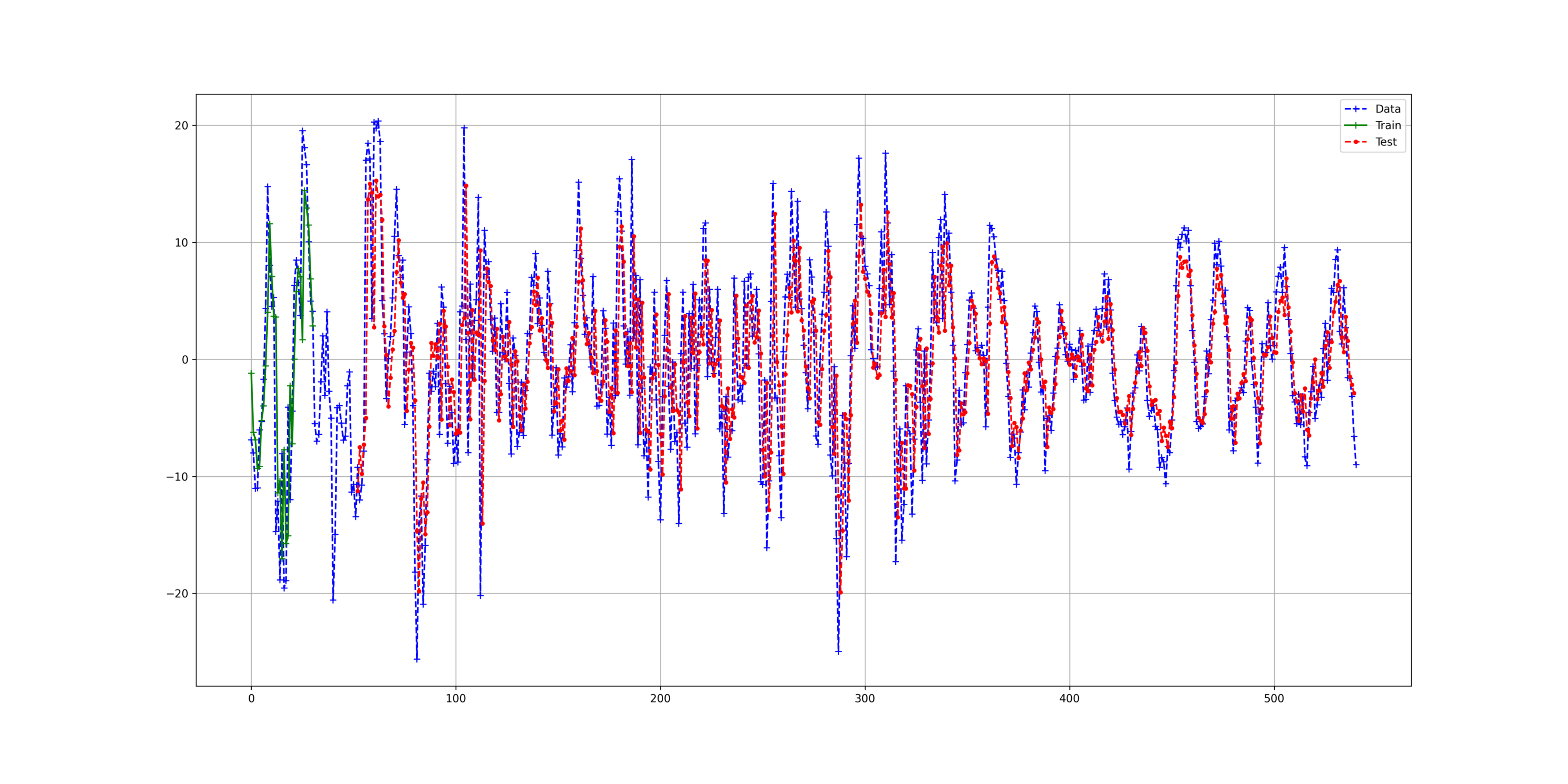
Table 1: Results of the different RNN models, showing the MAE and MSE metrics

表1：不同的RNN模型的结果，显示了MAE和MSE指标

        Name    | MAE Train | MSE Train | MAE Test | MSE Test
--------------------------------------------------------------------
            GRU |   4.24    |   34.11   |   4.15   |   31.47 
           LSTM |   4.26    |   34.54   |   4.16   |   31.64 
      Stack_GRU |   4.19    |   33.89   |   4.17   |   32.01
      SimpleRNN |   4.21    |   34.07   |   4.18   |   32.41
           LSTM |   4.28    |   35.1    |   4.21   |   31.9
         Bi_GRU |   4.21    |   34.34   |   4.22   |   32.54
  Stack_Bi_LSTM |   4.45    |   36.83   |   4.24   |   32.22
        Bi_LSTM |   4.31    |   35.37   |   4.27   |   32.4
Stack_SimpleRNN |   4.4     |   35.62   |   4.27   |   33.94
      SimpleRNN |   4.44    |   35.94   |   4.31   |   34.37 
     Stack_LSTM |   4.51    |   36.78   |   4.4    |   34.28
 Stacked_Bi_GRU |   4.56    |   37.32   |   4.45   |   35.34
       CNN_LSTM |   5.01    |   45.85   |   4.55   |   36.29
        CNN_GRU |   5.05    |   46.25   |   4.66   |   37.17 
  CNN_Stack_GRU |   5.07    |   45.92   |   4.7    |   38.64

The Table 1 shows the mean absolute error (MAE) and the mean squared error (MSE) for the train set and the test set for the RNN family. The GRU shows the best result on the test set with an MAE of 4.15 and an MSE of 31.47.

表1显示了RNN系列的火车和测试装置的平均绝对误差(MAE)和均方误差(MSE)。 GRU在测试集上显示最佳结果，MAE为4.15，MSE为31.47。

讨论区 (Discussion)

The results are good and reproduced the lightcurves of the different stars (see notebook). However, the fluctuations are not perfectly reproduced, the peaks do not have the same intensity and the flux is slightly shifted. A potential correction could be made via the attention mechanisms (Transformers[10]). Another way is to tune the models, the number of layers (stack), the number of units (cells), the combination of different RNN algorithms, new loss function or activation function, etc.

结果很好，再现了不同恒星的光曲线(请参阅笔记本)。 但是，波动不能完美地再现，峰的强度不同，通量也略有偏移。 潜在的纠正可以通过注意力机制(Transformers [10])进行。 另一种方法是调整模型，层数(堆栈)，单位数(单元)，不同RNN算法的组合，新的损失函数或激活函数等。

结论 (Conclusion)

This article shows the possibilities of combining so-called artificial intelligence methods with time series. The power of memory algorithms (RNN, LSTM, GRU) makes it possible to accurately reproduce sporadic fluctuations of events. In our case, the stellar flux exhibited quite strong and marked fluctuations that the methods have been able to capture.

本文展示了将所谓的人工智能方法与时间序列相结合的可能性。 记忆算法(RNN，LSTM，GRU)的强大功能使准确地再现事件的零星波动成为可能。 在我们的案例中，恒星通量表现出很强的明显波动，这些方法已经能够捕获这些波动。

This study shows that time series are no longer reserved for statistical methods such as the ARIMA[4] model.

这项研究表明，时间序列不再保留给ARIMA [4]模型之类的统计方法。