一元线性回归—实验部分
1. 一元线性回归
1.1 梯度下降法
首先载入数据,这里我们用到的是numpy库中的函数:
n
u
m
p
y
.
g
e
n
f
r
o
m
t
x
t
(
f
n
a
m
e
,
d
t
y
p
e
,
d
e
l
i
m
i
t
e
r
.
.
.
)
numpy.genfromtxt(fname,dtype,delimiter…)
numpy.genfromtxt(fname,dtype,delimiter...)
f
n
a
m
e
fname
fname可以表示文件名,文件路径等,
d
t
y
p
e
dtype
dtype表示数组的数据类型,
d
e
l
i
m
e
t
e
r
delimeter
delimeter表示分割数据的字符串,比如:,
下面我们就导入数据集,并查看:
代码:
import numpy as np
from numpy import genfromtxt
data=np.genfromtxt('data.csv',delimiter=',')
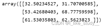
data[:3,]
结果:
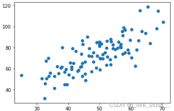
然后我们绘制散点图:
xdata=data[:,0]
ydata=data[:,1]
import matplotlib.pyplot as plt
plt.scatter(xdata,ydata)
plt.show()
结果:
然后我们可以求相关系数:
复习一下相关系数的公式:r
x
y
=
∑
(
X
−
X
‾
)
(
Y
−
Y
‾
)
∑
(
X
−
X
‾
)
2
∑
(
Y
−
Y
‾
)
2
r_{xy}=\frac{\sum(X-\overline{X})(Y-\overline{Y})}{\sqrt{\sum{(X-\overline{X}})^2\sum(Y-\overline{Y})^2}}
rxy=∑(X−X)2∑(Y−Y)2∑(X−X)(Y−Y)
其中的r
x
y
r_{xy}
rxy 越接近 1 ,说明具有线性特征
代码:
sumx=0
sumy=0
Numerator=0
denominatorX=0
denominatorY=0
for i in range(len(xdata)):
sumx=sumx+xdata[i]
sumy=sumy+ydata[i]
averX=sumx/len(xdata)
averY=sumy/len(ydata)
for i in range(len(xdata)):
Numerator = Numerator+(xdata[i]-averX)*(ydata[i]-averY)
denominatorX = denominatorX+(xdata[i]-averX)**2
denominatorY = denominatorY+(ydata[i]-averY)**2
rxy = Numerator/(np.sqrt(denominatorX*denominatorY))
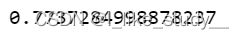
print(rxy)
求的结果:
接下来,就是进行梯度下降法求最小损失,以及参数
先来复习一下一元线性回归的相关知识:
- 定义假设函数:
h
y
p
o
t
h
e
s
i
s
:
h
θ
(
x
)
=
θ
0
+
θ
1
x
hypothesis:h_{\theta}(x)=\theta_0+\theta_1x
hypothesis:hθ(x)=θ0+θ1x
- 定义损失函数:
C
o
s
t
F
u
n
c
t
i
o
n
:
J
(
θ
0
,
θ
1
)
=
1
2
m
∑
i
=
0
m
(
h
θ
(
x
(
i
)
)
−
y
(
i
)
)
2
Cost~Function : J(\theta_0,\theta_1)=\frac{1}{2m}\sum_{i=0}^{m}(h_{\theta}(x^{(i)})-y^{(i)})^2
Cost Function:J(θ0,θ1)=2m1i=0∑m(hθ(x(i))−y(i))2
- 进行梯度下降:
r
e
p
e
a
t
u
n
t
i
l
c
o
n
v
e
r
g
e
n
c
e
{
θ
j
:
=
θ
j
−
∂
∂
θ
j
J
(
θ
0
,
θ
1
)
,
f
o
r
j
=
0
o
r
1
}
repeat~~until~~convergence\{ \\ \theta_j:=\theta_j-\frac{\partial}{\partial\theta_j}J(\theta_0,\theta_1),for~~j~=0~or~1 \\ \}
repeat until convergence{θj:=θj−∂θj∂J(θ0,θ1),for j =0 or 1}
代码:
# 定义假设函数
def hypothesis(theta0,theta1,x):
return theta0+theta1*x
# 定义损失函数
def costFunction(theta0,theta1,xdata,ydata):
totalError=0
for i in range(len(xdata)):
totalError+=(ydata[i]-hypothesis(theta0,theta1,xdata[i]))
return totalError/(2*len(xdata))
# 定义梯度下降函数
def gradient_descent_run(theta0,theta1,learn_rate,xdata,ydata,epochs):
m=len(xdata) # 数据集长度
#下面进行epochs次迭代:
for i in range(epochs):
theta0_gradient=0
theta1_gradient=0
for j in range(0,len(xdata)):
theta0_gradient+=(1/m)*(hypothesis(theta0,theta1,xdata[j])-ydata[j])
theta1_gradient+=(1/m)*(hypothesis(theta0,theta1,xdata[j])-ydata[j])*xdata[j]
theta0=theta0-theta0_gradient*learn_rate
theta1=theta1-theta1_gradient*learn_rate
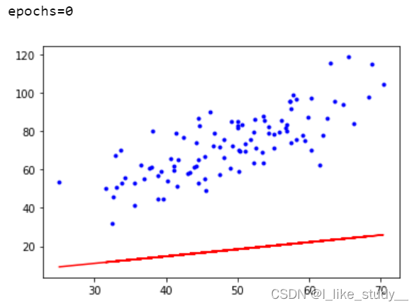
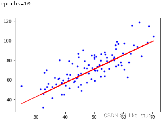
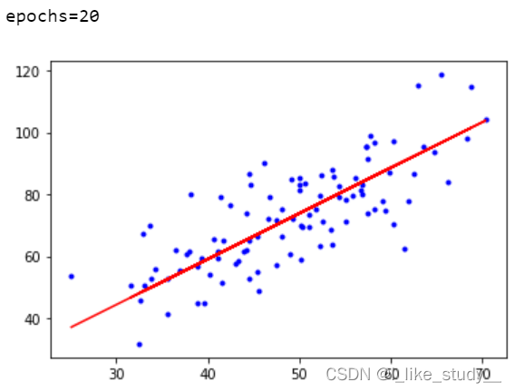
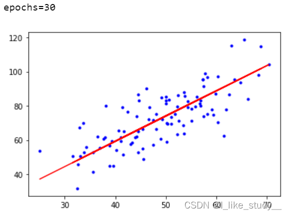
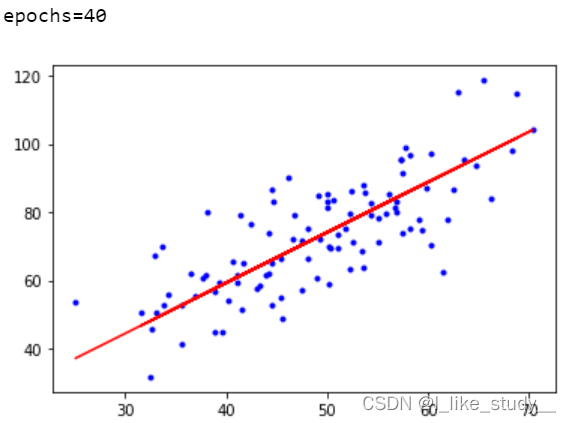
if i%10==0:
print("epochs={}".format(i))
plt.plot(xdata,ydata,'b.')
plt.plot(xdata,theta1*xdata+theta0,'r')
plt.show()
return theta0,theta1
#学习率
lr = 0.0001
# 截距
theta0 = 0
# 斜率
theta1 = 0
# 最大迭代次数
epochs = 50
theta0,theta1=gradient_descent_run(theta0,theta1,lr,xdata,ydata,epochs)
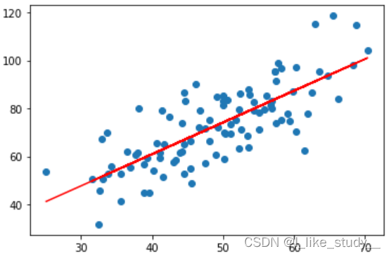
结果:
1.2 sklearn一元线性回归
先来看一下
s
k
l
e
a
r
n
.
l
i
n
e
a
r
_
m
o
d
e
l
.
L
i
n
e
a
r
R
e
g
r
e
s
s
i
o
n
(
)
sklearn.linear\_model.LinearRegression()
sklearn.linear_model.LinearRegression()的格式:
L
i
n
e
a
r
R
e
g
r
e
s
s
i
o
n
(
f
i
t
_
i
n
t
e
r
c
e
p
t
,
n
o
r
m
a
l
i
z
e
,
c
o
p
y
_
X
,
n
_
j
o
b
s
)
f
i
t
_
i
n
t
e
r
c
e
p
t
:
是
否
计
算
结
局
,
默
认
t
r
u
e
n
o
r
m
a
l
i
z
e
:
是
否
被
中
心
化
,
默
认
f
a
l
s
e
c
o
p
y
_
X
:
默
认
t
r
u
e
,
否
则
X
会
被
改
写
n
_
j
o
b
s
:
默
认
为
1
,
表
示
使
用
一
个
C
P
U
,
若
为
−
1
,
表
示
使
用
所
有
C
P
U
LinearRegression(fit\_intercept,normalize,copy\_X,n\_jobs) \\ fit\_intercept:是否计算结局,默认 true \\ normalize:是否被中心化,默认false \\ copy\_X:默认true,否则X会被改写 \\ n\_jobs:默认为1,表示使用一个CPU,若为-1,表示使用所有CPU
LinearRegression(fit_intercept,normalize,copy_X,n_jobs)fit_intercept:是否计算结局,默认truenormalize:是否被中心化,默认falsecopy_X:默认true,否则X会被改写n_jobs:默认为1,表示使用一个CPU,若为−1,表示使用所有CPU
调用方法:
c
o
e
f
_
:
训
练
后
的
输
入
端
模
型
系
数
,
如
果
y
值
有
两
列
,
就
是
一
个
2
D
的
a
r
r
a
y
coef\_:训练后的输入端模型系数,如果y值有两列,就是一个2D的array
coef_:训练后的输入端模型系数,如果y值有两列,就是一个2D的array
i
n
t
e
r
c
e
p
t
:
截
距
intercept_:截距
intercept:截距
p
r
e
d
i
c
t
(
x
)
:
预
测
数
据
predict(x):预测数据
predict(x):预测数据
s
c
o
r
e
:
评
估
score:评估
score:评估
示例:
import numpy as np
from sklearn.linear_model import LinearRegression
import matplotlib.pyplot as plt
# 导入数据
data=np.genfromtxt("data.csv",delimiter=',')
# 修改维度
x_data=data[:,0,np.newaxis]
y_data=data[:,1,np.newaxis]
# 建立模型
model=LinearRegression()
model.fit(x_data,y_data)
#绘制图像
plt.scatter(x_data,y_data)
plt.plot(x_data,model.predict(x_data),'r')
plt.show()
结果: