If you’re just starting out in Machine Learning, chances are you’ll be undertaking a classification project. As a beginner, I built an SMS spam classifier but did a ton of research to know where to start. In this article, I’ll walk you through my project in 10 steps to make it easier for you to build your first spam classifier using Tf-IDF Vectorizer, and the Naïve Bayes model!

如果您刚刚开始学习机器学习，那么您很可能会进行分类项目。 作为一个初学者，我建立了一个SMS垃圾邮件分类器，但进行了大量研究以了解从何开始。 在本文中，我将分10个步骤逐步介绍我的项目，以使您更轻松地使用Tf-IDF Vectorizer和NaïveBayes模型构建第一个垃圾邮件分类器！

1.加载并简化数据集 (1. Load and simplify the dataset)

Our SMS text messages dataset has 5 columns if you read it in pandas: v1 (containing the class labels ham/spam for each text message), v2 (containing the text messages themselves), and three Unnamed columns which have no use. We’ll rename the v1 and v2 columns to class_label and message respectively while getting rid of the rest of the columns.

如果您以熊猫阅读，我们的SMS短信数据集有5列：v1(每个短信包含类别标签ham / spam)，v2(包含短信本身)和三个无用的未命名列。 我们将第1版和第2版列分别重命名为class_label和message，而除去其余的列。

import pandas as pd
df = pd.read_csv(r'spam.csv',encoding='ISO-8859-1')
df.rename(columns = {'v1':'class_label', 'v2':'message'}, inplace = True)
df.drop(['Unnamed: 2', 'Unnamed: 3', 'Unnamed: 4'], axis = 1, inplace = True)df

Check out the fact that ‘5572 rows x 2 columns’ means that our dataset has 5572 text messages!

看看“ 5572行x 2列”这一事实意味着我们的数据集包含5572条文本消息！

2.浏览数据集：条形图 (2. Explore the dataset: Bar Chart)

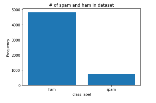
It’s a good idea to carry out some Exploratory Data Analysis (EDA) in a classification problem to visualize, get some information out of, or find any issues with your data before you start working with it. We’ll look at how many spam/ham messages we have and create a bar chart for it.

在开始处理分类问题之前，最好对分类问题进行一些探索性数据分析(EDA)以可视化，从中获取一些信息或发现任何问题。 我们将查看有多少垃圾邮件/火腿邮件，并为其创建条形图。

#exploring the datasetdf['class_label'].value_counts()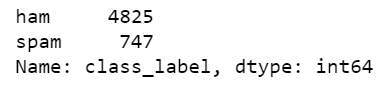

Our dataset has 4825 ham messages and 747 spam messages. This is an imbalanced dataset; the number of ham messages is much higher than those of spam! This can potentially cause our model to be biased. To fix this, we could resample our data to get an equal number of spam/ham messages.

我们的数据集包含4825个火腿邮件和747垃圾邮件。 这是一个不平衡的数据集； 火腿邮件的数量远高于垃圾邮件！ 这可能会导致我们的模型出现偏差。 为了解决这个问题，我们可以对数据重新采样以获取相同数量的垃圾邮件/火腿邮件。

To generate our bar chart, we use NumPy and pyplot from Matplotlib.

为了生成条形图，我们使用Matplotlib中的NumPy和pyplot。

3.探索数据集：词云 (3. Explore the dataset: Word Clouds)

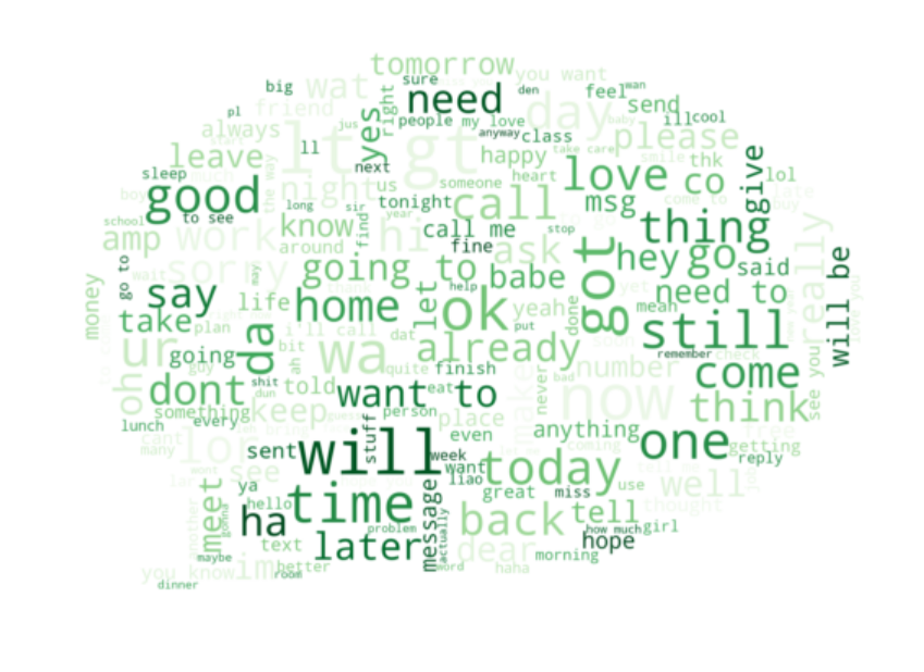
For my project, I generated word clouds of the most frequently occurring words in my spam messages.

对于我的项目，我生成了垃圾邮件中最常出现的单词的单词云。

First, we’ll filter out all the spam messages from our dataset. df_spam is a DataFrame that contains only spam messages.

首先，我们将从数据集中过滤掉所有垃圾邮件。 df_spam是仅包含垃圾邮件的DataFrame。

df_spam = df[df.class_label=='spam']df_spam

Next, we’ll convert our DataFrame to a list, where every element of that list will be a spam message. Then, we’ll join each element of our list into one big string of spam messages. The lowercase form of that string is the required format needed for our word cloud creation.

接下来，我们将DataFrame转换为一个列表，该列表中的每个元素都是垃圾邮件。 然后，我们将列表中的每个元素加入一大串垃圾邮件中。 该字符串的小写形式是创建词云所需的必需格式。

spam_list= df_spam['message'].tolist()filtered_spam = filtered_spam.lower()

Finally, we’ll import the relevant libraries and pass in our string as a parameter:

最后，我们将导入相关的库并将字符串作为参数传递：

import os
from wordcloud import WordCloud
from PIL import Imagecomment_mask = np.array(Image.open("comment.png"))
#create and generate a word cloud image
wordcloud = WordCloud(max_font_size = 160, margin=0, mask = comment_mask, background_color = "white", colormap="Reds").generate(filtered_spam)

After displaying it:

显示后：

Pretty cool, huh? The most common words in spam messages in our dataset are ‘free,’ ‘call now,’ ‘to claim,’ ‘have won,’ etc.

太酷了吧？ 在我们的数据集中，垃圾邮件中最常见的单词是“免费”，“立即致电”，“声明”，“赢得”等。

For this word cloud, we needed the Pillow library only because I’ve used masking to create that nice speech bubble shape. If you want it in square form, omit the mask parameter.

对于这个词云，我们仅需要Pillow库是因为我使用了遮罩来创建漂亮的语音气泡形状。 如果要以正方形形式使用，请省略mask参数。

Similarly, for ham messages:

同样，对于火腿消息：

4.处理不平衡的数据集 (4. Handle imbalanced datasets)

To handle imbalanced data, you have a variety of options. I got a pretty good f-measure in my project even with unsampled data, but if you want to resample, see this.

要处理不平衡的数据，您有多种选择。 即使使用未采样的数据，我在项目中也获得了相当不错的f度量，但是如果您想重新采样，请参阅此 。

5.分割数据集 (5. Split the dataset)

First, let’s convert our class labels from string to numeric form:

首先，让我们将类标签从字符串转换为数字形式：

df['class_label'] = df['class_label'].apply(lambda x: 1 if x == 'spam' else 0)

In Machine Learning, we usually split our data into two subsets — train and test. We feed the train set along with the known output values for it (in this case, 0 or 1 corresponding to spam or ham) to our model so that it learns the patterns in our data. Then we use the test set to get the model’s predicted labels on this subset. Let’s see how to split our data.

在机器学习中，我们通常将数据分为两个子集：训练和测试。 我们将训练集及其已知的输出值(在这种情况下为0或1，对应于垃圾邮件或火腿)输入模型，以便它学习数据中的模式。 然后，我们使用测试集在此子集上获取模型的预测标签。 让我们看看如何拆分数据。

First, we import the relevant module from the sklearn library:

首先，我们从sklearn库中导入相关模块：

from sklearn.model_selection import train_test_split

And then we make the split:

然后我们进行拆分：

x_train, x_test, y_train, y_test = train_test_split(df['message'], df['class_label'], test_size = 0.3, random_state = 0)

Let’s now see how many messages we have for our test and train subsets:

现在，让我们看看我们的测试和训练子集有多少条消息：

print('rows in test set: ' + str(x_test.shape))
print('rows in train set: ' + str(x_train.shape))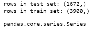

So we have 1672 messages for testing, and 3900 messages for training!

因此，我们有1672条消息用于测试，3900条消息用于培训！

6.应用Tf-IDF矢量化器进行特征提取 (6. Apply Tf-IDF Vectorizer for feature extraction)

Our Naïve Bayes model requires data to be in either Tf-IDF vectors or word vector count. The latter is achieved using Count Vectorizer, but we’ll obtain the former through using Tf-IDF Vectorizer.

我们的朴素贝叶斯模型要求数据必须在Tf-IDF向量或单词向量计数中。 后者是使用Count Vectorizer实现的，但我们将使用Tf-IDF Vectorizer获得前者。

TF-IDF Vectorizer creates Tf-IDF values for every word in our text messages. Tf-IDF values are computed in a manner that gives a higher value to words appearing less frequently so that words appearing many times due to English syntax don’t overshadow the less frequent yet more meaningful and interesting terms.

TF-IDF矢量化器为文本消息中的每个单词创建Tf-IDF值。 Tf-IDF值的计算方式是为出现频率较低的单词赋予较高的值，以使由于英语语法而出现多次的单词不会掩盖频率较低但更有意义和有趣的术语。

lst = x_train.tolist()
vectorizer = TfidfVectorizer(
input= lst ,  # input is the actual text
lowercase=True,      # convert to lowercase before tokenizing
stop_words='english' # remove stop words
)features_train_transformed = vectorizer.fit_transform(list) #gives tf idf vector for x_train
features_test_transformed  = vectorizer.transform(x_test) #gives tf idf vector for x_test

7.训练我们的朴素贝叶斯模型 (7. Train our Naive Bayes Model)

We fit our Naïve Bayes model, aka MultinomialNB, to our Tf-IDF vector version of x_train, and the true output labels stored in y_train.

我们将我们的朴素贝叶斯模型(也称为MultinomialNB)拟合到我们的Tf-IDF矢量版本x_train，并将真实输出标签存储在y_train中。

from sklearn.naive_bayes import MultinomialNB
# train the model
classifier = MultinomialNB()
classifier.fit(features_train_transformed, y_train)

8.检查准确性，并进行f测度 (8. Check out the accuracy, and f-measure)

It’s time to pass in our Tf-IDF matrix corresponding to x_test, along with the true output labels (y_test), to find out how well our model did!

现在该传递与x_test对应的Tf-IDF矩阵以及真实的输出标签(y_test)，以了解我们的模型的效果如何！

First, let’s see the model accuracy:

首先，让我们看看模型的准确性：

print("classifier accuracy {:.2f}%".format(classifier.score(features_test_transformed, y_test) * 100))

Our accuracy is great! However, it’s not a great indicator if our model becomes biased. Hence we perform the next step.

我们的准确性非常好！ 但是，如果我们的模型出现偏差，这并不是一个很好的指标。 因此，我们执行下一步。

9.查看混淆矩阵和分类报告 (9. View the confusion matrix and classification report)

Let’s now look at our confusion matrix and f-measure scores to confirm if our model is doing OK or not:

现在，让我们看一下混淆矩阵和f-measure得分，以确认我们的模型是否正常：

labels = classifier.predict(features_test_transformed)
from sklearn.metrics import f1_score
from sklearn.metrics import confusion_matrix
from sklearn.metrics import accuracy_score
from sklearn.metrics import classification_reportactual = y_test.tolist()
predicted = labels
results = confusion_matrix(actual, predicted)
print('Confusion Matrix :')
print(results)
print ('Accuracy Score :',accuracy_score(actual, predicted))
print ('Report : ')
print (classification_report(actual, predicted) )
score_2 = f1_score(actual, predicted, average = 'binary')
print('F-Measure: %.3f' % score_2)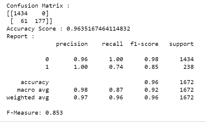

We have an f-measure score of 0.853, and our confusion matrix shows that our model is making only 61 incorrect classifications. Looks pretty good to me ?

我们的f测度得分为0.853，而混淆矩阵表明我们的模型仅进行了61个错误的分类。 对我来说看起来不错?

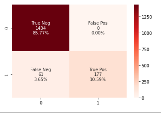
10.混淆矩阵的热图(可选) (10. Heatmap for our Confusion Matrix (Optional))

You can create a heatmap using the seaborn library to visualize your confusion matrix. The code below does just that.

您可以使用seaborn库创建热图以可视化混淆矩阵。 下面的代码就是这样做的。

And that’s it to make your very own spam classifier! To summarize, we imported the dataset and visualized it. Then we split it into train/test and converted it into Tf-IDF vectors. Finally, we trained our Naive Bayes model, and saw the results! You could take this a step further and deploy it as a web app if you like.

这就是您自己的垃圾邮件分类器！ 总而言之，我们导入了数据集并将其可视化。 然后我们将其拆分为训练/测试，并将其转换为Tf-IDF向量。 最后，我们训练了我们的朴素贝叶斯模型，并看到了结果！ 如果愿意，您可以进一步将它部署为Web应用程序。

参考资料/资源： (References/Resources:)

[1]D. T, Confusion Matrix Visualization (2019), https://medium.com/@dtuk81/confusion-matrix-visualization-fc31e3f30fea

[1] D.T，混淆矩阵可视化(2019)， https://medium.com/@dtuk81/confusion-matrix-visualization-fc31e3f30fea

1. C. Vince,Naive Bayes Spam Classifier (2018), https://www.codeproject.com/Articles/1231994/Naive-Bayes-Spam-Classifier

   C.文斯 朴素贝叶斯垃圾邮件分类器(2018)， https://www.codeproject.com/Articles/1231994/Naive-Bayes-Spam-Classifier

2. H. Attri,Feature Extraction using TF-IDF algorithm (2019), https://medium.com/@hritikattri10/feature-extraction-using-tf-idf-algorithm-44eedb37305e

   H. Attri， 使用TF-IDF算法进行特征提取(2019)， https://medium.com/@hritikattri10/feature-extraction-using-tf-idf-algorithm-44eedb37305e

3. A. Bronshtein, Train/Test Split and Cross Validation in Python (2017), https://towardsdatascience.com/train-test-split-and-cross-validation-in-python-80b61beca4b6

   A.Bronshtein，《 Python中的Train / Test拆分和交叉验证》(2017年)， https ：//towardsdatascience.com/train-test-split-and-cross-validation-in-python-80b61beca4b6

4. Dataset: https://www.kaggle.com/uciml/sms-spam-collection-dataset

   数据集 ： https : //www.kaggle.com/uciml/sms-spam-collection-dataset

5. Full code: https://github.com/samimakhan/Spam-Classification-Project/tree/master/Naive-Bayes

   完整代码 ： https : //github.com/samimakhan/Spam-Classification-Project/tree/master/Naive-Bayes