今天主要想说的是,分形中的差分盒子维数的原理,基于分形的基础概念就不在这里说啦.
分形维数可以用于定量描述图像表面的空间复杂程度,能够定量的表现图像的纹理特征. 采用不同的维数进行纹理特征描述时,精度有所区别,我们今天主要来说一下比较简单的盒子维.
1.差分盒子维数
Gangepain 和 Roques-Carms 在1986年提出基于盒计数(Box-counting)的分形维数,通过计算覆盖图像表面的最小盒子数来度量.
说得详细一点:将一幅大小为
注:一般灰度图像的灰度级为 L = 256.若在第
覆盖整个盒子的数为
由此可求分形维数D为:
式中:
通过改变网格
2.实验
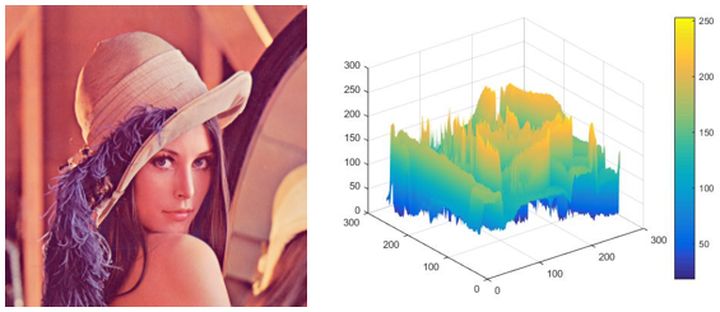
我们先来看一下,将灰度图像看作三维物体的表面灰度集是怎么样呢?
① 实现灰度图像的表面灰度集,采用matlab程序,如下:
function Show_GraySurface(filename)

%   把一幅图像看成三维空间的曲面,
%   像素的位置(x,y)构成xoy坐标面,
%   像素的灰度值看成z轴的值由此构成灰度曲面
    picture_dir = 'D:Matlabworktest';
    I = imread([picture_dir,filename]);
        if (length(size(I)) > 2)
            I = rgb2gray(I);
        end
    M = size(I,1);
    Temp = diag(1:256)*ones(256,256);
    x = reshape(Temp.',1,M*M);
    y = reshape(Temp,1,M*M);
    z = reshape(I,1,M*M);
    tri = delaunay(x,y);
    trisurf(tri,x,y,z);
    shading interp
    view(3);grid on;colorbar

end
附加:python程序
import cv2
import numpy as np
import matplotlib.pyplot as plt


def surface(img):

    X = np.arange(0, 363, 1) # cols of the image
    Y = np.arange(0, 480, 1) # rows of the image

    X,Y = np.meshgrid(X,Y)   # extending points


    Z = np.array(img)      #2 dimension

    fig, ax = plt.subplots(subplot_kw = {"projection": "3d"})

    surf = ax.plot_surface(X, Y, Z, cmap = "rainbow", linewidth = 0, antialiased = False)

    ax.contour(X, Y, Z, zdir = 'z', offset = 75, cmap = plt.get_cmap('rainbow'))  # projection

    fig.colorbar(surf)  # colorbar

    plt.show()


if __name__ == "__main__":

    img = cv2.imread("3.jpg", 0)

    surface(img)
注:matlab程序中,图像大小256 x 256.效果如下:
② 计算差分盒维数,采用Python程序.
★ 主程序文件:main.py
import cv2
from DBC import Fractal

src = cv2.imread("D5.jpg", cv2.IMREAD_UNCHANGED)

# create an object
obj = Fractal()

#linear fitting for solveing differential box dimension(DBC)
obj.execute(src)
★ 子程序文件:DBC.py
import numpy as np
import cv2
import math
from matplotlib import pyplot as plt


class Fractal():


    def __init__(self):
        pass

    # method of image graying
    def gray(self, src):

        gray_img = np.uint8(src[:,:, 0] * 0.144 + src[:, :, 1] * 0.587 + src[:, :, 2] * 0.299)

        # cla_img = cv2.bilateralFilter(gray_img, 3, 64, 64)


        # #clahe processing
        # clahe = cv2.createCLAHE(clipLimit = 3, tileGridSize = (32, 32))
        # cla_img = clahe.apply(bil_img)

        return gray_img


    #  differential box dimension counting (DBC)
    def differential_box_counting (self, gray_img):

        h, w = gray_img.shape[:2]
        M = min(h,w)

        Nr = []

        for s in range(2,M//2+1,1):         # the box side length: 2 ~ M//2
            H = 255*s/M                     # high of the box
            box_num = 0                     # initialization of the box number
            for row in range(h//s):         # h//s: the number of rows in the box;  w//s: the number of columns in the box
                for col in range(w//s):
                    nr = math.ceil((np.max(gray_img[row*s:(row+1)*s, col*s:(col+1)*s])-np.min(gray_img[row*s:(row+1)*s, col*s:(col+1)*s]))/H +1)
                    box_num += nr
            Nr.append(box_num)

        return Nr,M


    def least_squares(self, x , y):

        """
        (1) input datesets of x and y
        (2) the straight line is fitted by Least-square method
        (3) output a coefficient(w), intercept(b) and coefficient of determination (r)
        (4) the fitting straight line : y = wx + b
        """
        x_ = x.mean()
        y_ = y.mean()

        m1 = np.zeros(1)
        m2 = np.zeros(1)
        m3 = np.zeros(1)

        k1 = np.zeros(1)
        k2 = np.zeros(1)
        k3 = np.zeros(1)


        for i in np.arange(len(x)):

            m1 += (x[i] - x_)* y[i]
            m2 += np.square(x[i])
            m3 += x[i]

            k1 += (x[i]-x_) * (y[i]-y_)
            k2 += np.square(x[i] - x_)
            k3 += np.square(y[i] - y_)

        w = m1/(m2 - 1/len(x) * np.square(m3))
        b = y_ - w * x_
        r = k1 / np.sqrt(k2 * k3)

        return w, b, r


    def plot_line(self, x, y, w, b, r):


        # print(w, b, r ** 2)
        y_pred = w * x + b


        # create a fig and an axes
        fig, ax = plt.subplots(figsize = (10, 5))

        # fontsyle: SimHei(黑体),support chinese
        plt.rcParams['font.sans-serif'] = ['SimHei']

        ax.plot(x, y, 'co', markersize = 6, label = 'scatter datas')
        ax.plot(x, y_pred, 'r-', linewidth = 2, label = 'y = %.4fx + %.4f' %(w, b))

        # set xlim and yxlim
        ax.set_aspect("0.5")
        ax.set_xlim(1, 6)
        ax.set_ylim(2, 12)

        # set x_ticks and y_ticks
        ax.tick_params(labelsize = 16)
        labels = ax.get_xticklabels() + ax.get_yticklabels()
        [label.set_fontname('Times New Roman') for label in labels]

        # create grids
        ax.grid(which = "major", axis = "both")

        # display labels
        font1 = {'family': 'Times New Roman', 'weight': 'normal', 'size': 16}
        ax.legend(prop = font1)

        #set x_label and y_label
        font2 = {'family': 'Times New Roman', 'weight': 'normal', 'size': 20}
        ax.set_xlabel("ln 1/r", fontdict = font2)
        ax.set_ylabel("ln Nr", fontdict = font2)

        # set a position of "R^2"
        ax.text(3.5, 7.8, 'R^2 = %.4f' % float(r * r), fontdict = font1,
                verticalalignment='center', horizontalalignment ='left', rotation=0)

        plt.savefig("line.jpg", dpi = 300, bbox_inches = "tight")

        plt.show()


    def execute(self, img):

        gray_img = self.gray(img)

        Nr, M = self.differential_box_counting(gray_img)

        x = np.log([round(M/s) for s in range(2,M//2+1,1)])
        y = np.log(Nr)

        #fitting a straight line
        w, b, r = self.least_squares(x, y)

        self.plot_line(x, y, w, b, r)
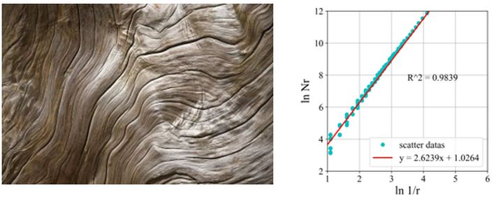
我们来看一下效果图:用最小二乘法进行拟合,斜率就是我们需要的维数.
# 其实最小二乘法,也可以通过sklearn库直接调用.

import cv2
import numpy as np
import math
from matplotlib import pyplot as plt
from sklearn import linear_model
from sklearn.metrics import r2_score

from numba import jit

@jit
def differential_box_counting (gray_img):
    # cv2.imshow("gray_img",gray_img)
    h, w = gray_img.shape[:2]
    M = min(h,w)

    Nr = []
    for s in range(2,M//2+1,1):         #盒子边长从2到图片最小尺寸的二分之一,每次边长加1
        H = 255*s/M        #盒子柱高l
        box_num = 0         #初始化盒子数
        for row in range(h//s):           #(h//s)为盒子的行数,(w//s)为盒子的列数
            for col in range(w//s):
                nr = math.ceil((np.max(gray_img[row*s:(row+1)*s, col*s:(col+1)*s])-np.min(gray_img[row*s:(row+1)*s, col*s:(col+1)*s]))/H +1)
                box_num += nr
        Nr.append(box_num)

    return Nr,M

def Least_squares():
    x = np.log([round(M/s) for s in range(2,M//2+1,1)])
    x = np.array(x).reshape((-1, 1))  # transform list to numpy.ndarray

    y = np.log(Nr)
    y = np.array(y).reshape((-1, 1))  # transform list to numpy.ndarray


    # Create linear regression object
    regr = linear_model.LinearRegression()  # is equivalent to  # regr = linear_model.Ridge(alpha = 0)

    # Train the model using the sets
    regr.fit(x, y)
    y_pred = regr.predict(x)

    # The coefficients
    print('Coefficients:   ', regr.coef_)

    #The intercept
    print('Intercept:  ', regr.intercept_)

    # The coefficient of determination: 1 is perfect prediction
    print('Coefficient of determination: %.8f'
      % r2_score(y, y_pred))

    plt.scatter(x, y,  color='black')
    plt.plot(x, y_pred, color='blue', linewidth=3)

    plt.show()

if __name__ == "__main__":

    gray_img = cv2.imread("D3.jpg", cv2.IMREAD_GRAYSCALE)

    # thresh = cv2.threshold(gray_img, 220, 255, cv2.THRESH_BINARY)[1]
    Nr,M = differential_box_counting(gray_img)

    Least_squares()
喜欢的话,给予鼓励,点个赞...
版权声明:本文为weixin_35717340原创文章,遵循CC 4.0 BY-SA版权协议,转载请附上原文出处链接和本声明。