1 简介

在计算机视觉中，基础矩阵（Fundamental matrix）F是一个3×3的矩阵，表达了立体像对的像点之间的对应关系。在对极几何中，对于立体像对中的一对同名点，它们的齐次化图像坐标分别为p与 p’，表示一条必定经过p’的直线（极线）。这意味着立体像对的所有同名点对都满足：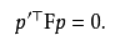
在这里插入图片描述
F矩阵中蕴含了立体像对的两幅图像在拍摄时相互之间的空间几何关系（外参数）以及相机检校参数（内参数），包括旋转、位移、像主点坐标和焦距。因为F矩阵的秩为2，并且可以自由缩放（尺度化），所以只需7对同名点即可估算出F的值。
基础矩阵这一概念由Q. T. Luong在他那篇很有影响力的博士毕业论文中提出。 [1] Faugeras则是在1992年发表的著作 [2] 中以上面的关系式给出了F矩阵的定义。尽管Longuet-Higgins提出的本质矩阵也满足类似的关系式，但本质矩阵中并不蕴含相机检校参数。本质矩阵与基础矩阵之间的关系可由下式表达：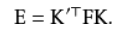
在这里插入图片描述
其中K和K’分别为两个相机的内参数矩阵。

2 基础矩阵

2.1对极几何

对极几何概念
对极几何实际上是“两幅图像之间的对极几何”，它是图像平面与以基线为轴的平面束的交的几何（这里的基线是指连接摄像机中心的直线），以下图为例：对极几何描述的是左右两幅图像(点x和x’对应的图像)与以CC’为轴的平面束的交的几何
在这里插入图片描述直线CC’为基线，以该基线为轴存在一个平面束，该平面束与两幅图像平面相交，下图给出了该平面束的直观形象，可以看到，该平面束中不同平面与两幅图像相交于不同直线；

上图中的灰色平面π，只是过基线的平面束中的一个平面（当然，该平面才是平面束中最重要的、也是我们要研究的平面）

2.2本质矩阵

设X在C， C’坐标系中的相对坐标分别p， p’，则有
根据三线共面有：

又有：

将其改写成：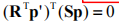

变化后得到：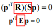

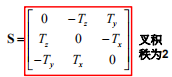
最后得到本质矩阵E在这里插入图片描述
本质矩阵描述了空间中的点在两个坐标系中的坐标对应关系。

2.3基础矩阵

根据前述， K 和 K’ 分别为两个相机的内参矩阵，有：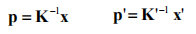
在这里插入图片描述
带入上式，我们可以得到：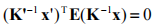

计算得到: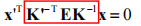

红色方框种的式子则为基础矩阵F:

基础矩阵描述了空间中的点在两个像平面中的坐标对应关系。可以用于: 1 简化匹配 2去除错配特征

2.4 8点算法估计基础矩阵F

八点估算
基本矩阵是由该方程定义的： x′TFx=0
其中x↔x′是两幅图像的任意一对匹配点。由于每一组点的匹配提供了计算F系数的一个线性方程，当给定至少7个点（3×3的齐次矩阵减去一个尺度，以及一个秩为2的约束），方程就可以计算出未知的F。我们记点的坐标为x=(x,y,1)T，x′=(x′,y′,1)T
又因为F为：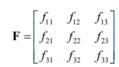
在这里插入图片描述
所以可得到方程：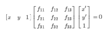

即相应方程式为

给定n组点的集合，我们有如下方程：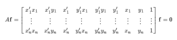

如果存在确定（非零）解，则系数矩阵A的秩最多是8。由于F是齐次矩阵，所以如果矩阵A的秩为8，则在差一个尺度因子的情况下解是唯一的。可以直接用线性算法解得。
如果由于点坐标存在噪声则矩阵AA的秩可能大于8（也就是等于9，由于A是n×9的矩阵）。这时候就需要求最小二乘解，这里就可以用SVD来求解，f的解就是系数矩阵A最小奇异值对应的奇异向量，也就是A奇异值分解后A=UDVT中矩阵V的最后一列矢量，这是在解矢量f在约束∥f∥下取∥Af∥最小的解。以上算法是解基本矩阵的基本方法，称为8点算法。
上述求解后的F不一定能满足秩为2的约束，因此还要在F的基础上加以约束。通过SVD分解可以解决，令F=UΣVT，则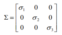
在这里插入图片描述
因为要秩为2，所以取最后一个元素设置为0，则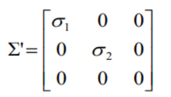

最终的解：

3 代码实现

3.1代码

1 sift提取特征
2 RANSAC去除错误点匹配
3 归一化8点算法估计基础矩阵

# -*- coding: utf-8 -*-
from PIL import Image
from numpy import *
from pylab import *
import numpy as np
from PCV.geometry import camera
from PCV.geometry import homography
from PCV.geometry import sfm
from PCV.localdescriptors import sift
# -*- coding: utf-8 -*-

# Read features
# 载入图像，并计算特征
im1 = array(Image.open('E:/picture/02/1.jpg'))
sift.process_image('E:/picture/02/1.jpg', 'im1.sift')
l1, d1 = sift.read_features_from_file('im1.sift')

im2 = array(Image.open('E:/picture/02/2.jpg'))
sift.process_image('E:/picture/02/2.jpg', 'im2.sift')
l2, d2 = sift.read_features_from_file('im2.sift')

# 匹配特征
matches = sift.match_twosided(d1, d2)
ndx = matches.nonzero()[0]

# 使用齐次坐标表示，并使用 inv(K) 归一化
x1 = homography.make_homog(l1[ndx, :2].T)
ndx2 = [int(matches[i]) for i in ndx]
x2 = homography.make_homog(l2[ndx2, :2].T)

x1n = x1.copy()
x2n = x2.copy()
print(len(ndx))

figure(figsize=(16,16))
sift.plot_matches(im1, im2, l1, l2, matches, True)
show()

# Don't use K1, and K2

#def F_from_ransac(x1, x2, model, maxiter=5000, match_threshold=1e-6):
def F_from_ransac(x1, x2, model, maxiter=5000, match_threshold=1e-6):
    """ Robust estimation of a fundamental matrix F from point
    correspondences using RANSAC (ransac.py from
    http://www.scipy.org/Cookbook/RANSAC).

    input: x1, x2 (3*n arrays) points in hom. coordinates. """

    from PCV.tools import ransac
    data = np.vstack((x1, x2))
    d = 20 # 20 is the original
    # compute F and return with inlier index
    F, ransac_data = ransac.ransac(data.T, model,
                                   8, maxiter, match_threshold, d, return_all=True)
    return F, ransac_data['inliers']

# find E through RANSAC
# 使用 RANSAC 方法估计 E
model = sfm.RansacModel()
F, inliers = F_from_ransac(x1n, x2n, model, maxiter=5000, match_threshold=1e-4)

print(len(x1n[0]))
print(len(inliers))

# 计算照相机矩阵（P2 是 4 个解的列表）
P1 = array([[1, 0, 0, 0], [0, 1, 0, 0], [0, 0, 1, 0]])
P2 = sfm.compute_P_from_fundamental(F)

# triangulate inliers and remove points not in front of both cameras
X = sfm.triangulate(x1n[:, inliers], x2n[:, inliers], P1, P2)

# plot the projection of X
cam1 = camera.Camera(P1)
cam2 = camera.Camera(P2)
x1p = cam1.project(X)
x2p = cam2.project(X)

figure()
imshow(im1)
gray()
plot(x1p[0], x1p[1], 'o')
#plot(x1[0], x1[1], 'r.')
axis('off')

figure()
imshow(im2)
gray()
plot(x2p[0], x2p[1], 'o')
#plot(x2[0], x2[1], 'r.')
axis('off')
show()

figure(figsize=(16, 16))
im3 = sift.appendimages(im1, im2)
im3 = vstack((im3, im3))

imshow(im3)

cols1 = im1.shape[1]
rows1 = im1.shape[0]
for i in range(len(x1p[0])):
    if (0<= x1p[0][i]<cols1) and (0<= x2p[0][i]<cols1) and (0<=x1p[1][i]<rows1) and (0<=x2p[1][i]<rows1):
        plot([x1p[0][i], x2p[0][i]+cols1],[x1p[1][i], x2p[1][i]],'c')
axis('off')
show()

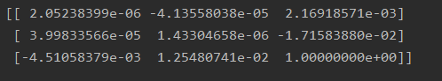
print(F)

x1e = []
x2e = []
ers = []
for i,m in enumerate(matches):
    if m>0: #plot([locs1[i][0],locs2[m][0]+cols1],[locs1[i][1],locs2[m][1]],'c')
        x1=int(l1[i][0])
        y1=int(l1[i][1])
        x2=int(l2[int(m)][0])
        y2=int(l2[int(m)][1])
        # p1 = array([l1[i][0], l1[i][1], 1])
        # p2 = array([l2[m][0], l2[m][1], 1])
        p1 = array([x1, y1, 1])
        p2 = array([x2, y2, 1])
        # Use Sampson distance as error
        Fx1 = dot(F, p1)
        Fx2 = dot(F, p2)
        denom = Fx1[0]**2 + Fx1[1]**2 + Fx2[0]**2 + Fx2[1]**2
        e = (dot(p1.T, dot(F, p2)))**2 / denom
        x1e.append([p1[0], p1[1]])
        x2e.append([p2[0], p2[1]])
        ers.append(e)
x1e = array(x1e)
x2e = array(x2e)
ers = array(ers)

indices = np.argsort(ers)
x1s = x1e[indices]
x2s = x2e[indices]
ers = ers[indices]
x1s = x1s[:20]
x2s = x2s[:20]

figure(figsize=(16, 16))
im3 = sift.appendimages(im1, im2)
im3 = vstack((im3, im3))

imshow(im3)

cols1 = im1.shape[1]
rows1 = im1.shape[0]
for i in range(len(x1s)):
    if (0<= x1s[i][0]<cols1) and (0<= x2s[i][0]<cols1) and (0<=x1s[i][1]<rows1) and (0<=x2s[i][1]<rows1):
        plot([x1s[i][0], x2s[i][0]+cols1],[x1s[i][1], x2s[i][1]],'c')
axis('off')
show()