1
Matlab:地理加权回归模型命令简介
在Matlab软件中,可以调用gwr.m来实现地理加权回归模型的参数过程,下面介绍 GWR 在Matlab中的实现过程:
“gwr.m”函数命令的调用方式如下所示:
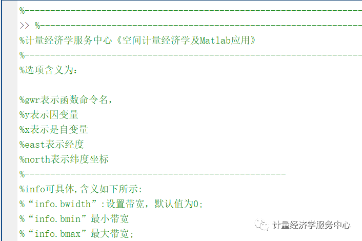
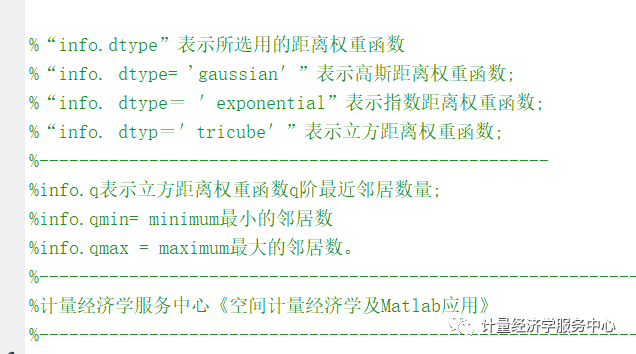
#%% 地理加权回归模型MATLAB程序代码如下>> help gwr PURPOSE: compute geographically weighted regression ---------------------------------------------------- USAGE: results = gwr(y,x,east,north,info) where: y = dependent variable vector x = explanatory variable matrix east = x-coordinates in space north = y-coordinates in space info = a structure variable with fields: info.bwidth = scalar bandwidth to use or zero for cross-validation estimation (default) info.bmin = minimum bandwidth to use in CV search info.bmax = maximum bandwidth to use in CV search defaults: bmin = 0.1, bmax = 20 info.dtype = 'gaussian' for Gaussian weighting (default) = 'exponential' for exponential weighting = 'tricube' for tri-cube weighting info.q = q-nearest neighbors to use for tri-cube weights (default: CV estimated) info.qmin = minimum # of neighbors to use in CV search info.qmax = maximum # of neighbors to use in CV search defaults: qmin = nvar+2, qmax = 4*nvar --------------------------------------------------- NOTE: res = gwr(y,x,east,north) does CV estimation of bandwidth --------------------------------------------------- RETURNS: a results structure results.meth = 'gwr' results.beta = bhat matrix (nobs x nvar) results.tstat = t-stats matrix (nobs x nvar) results.yhat = yhat results.resid = residuals results.sige = e'e/(n-dof) (nobs x 1) results.nobs = nobs results.nvar = nvars results.bwidth = bandwidth if gaussian or exponential results.q = q nearest neighbors if tri-cube results.dtype = input string for Gaussian, exponential weights results.iter = # of simplex iterations for cv results.north = north (y-coordinates) results.east = east (x-coordinates) results.y = y data vector --------------------------------------------------- See also: prt,plt, prt_gwr, plt_gwr to print and plot results --------------------------------------------------- References: Brunsdon, Fotheringham, Charlton (1996) Geographical analysis, pp. 281-298 --------------------------------------------------- NOTES: uses auxiliary function scoref for cross-validation ---------------------------------------------------选项含义为:
2
高斯距离权重函数地理加权回归模型
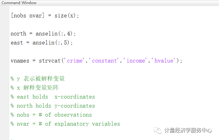
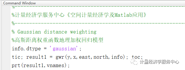
选择高斯距离权重函数进行地理加权回归模型代码如下:
%--------------------------------------------------------------------------%计量经济学服务中心《空间计量经济学及Matlab应用》%--------------------------------------------------------------------------%高斯距离权重函数地理加权回归模型% load the Anselin data set% 导入数据load anselin.dat;y = anselin(:,1);nobs = length(y);x = [ones(nobs,1) anselin(:,2:3)];[nobs nvar] = size(x);north = anselin(:,4);east = anselin(:,5);vnames = strvcat('crime','constant','income','hvalue');%--------------------------------------------------------------------------%计量经济学服务中心《空间计量经济学及Matlab应用》%--------------------------------------------------------------------------% Gaussian distance weighting%高斯距离权重函数地理加权回归模型info.dtype = 'gaussian'; tic; result1 = gwr(y,x,east,north,info); toc;prt(result1,vnames);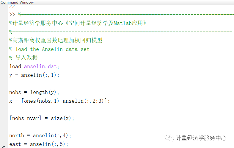
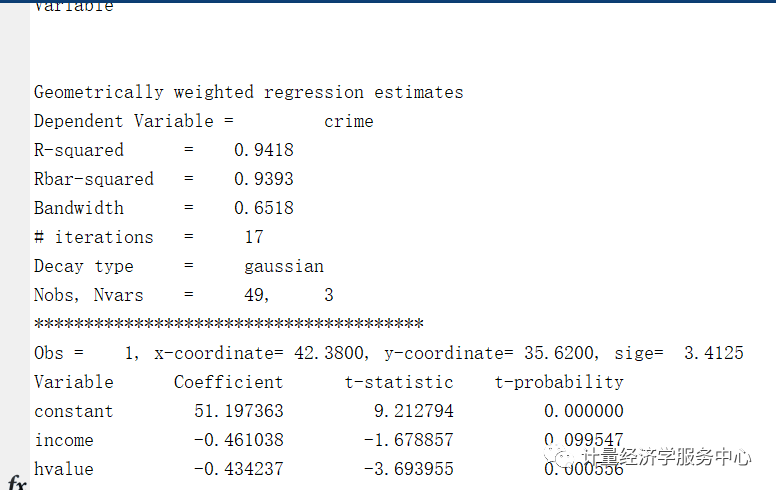
结果为:
14-49空间单元的参数估计结果不再展现,完整结果可以查看后面代码。
3
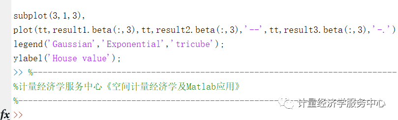
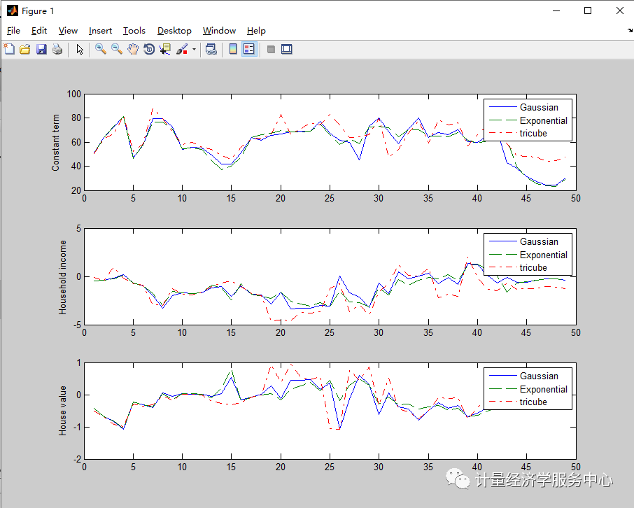
三种不同空间权重矩阵参数比较
命令为:
%--------------------------------------------------------------------------%计量经济学服务中心《空间计量经济学及Matlab应用》%--------------------------------------------------------------------------% plot results for comparison (see also plt)tt=1:nobs;subplot(3,1,1),plot(tt,result1.beta(:,1),tt,result2.beta(:,1),'--',tt,result3.beta(:,1),'-.');legend('Gaussian','Exponential','tricube');ylabel('Constant term');subplot(3,1,2),plot(tt,result1.beta(:,2),tt,result2.beta(:,2),'--',tt,result3.beta(:,2),'-.');legend('Gaussian','Exponential','tricube');ylabel('Household income');subplot(3,1,3),plot(tt,result1.beta(:,3),tt,result2.beta(:,3),'--',tt,result3.beta(:,3),'-.');legend('Gaussian','Exponential','tricube');ylabel('House value');%--------------------------------------------------------------------------%计量经济学服务中心《空间计量经济学及Matlab应用》%--------------------------------------------------------------------------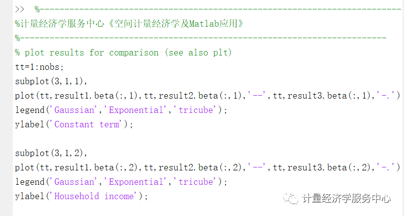
结果为:
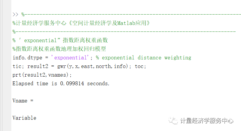
4
指数距离权重函数地理加权回归模型
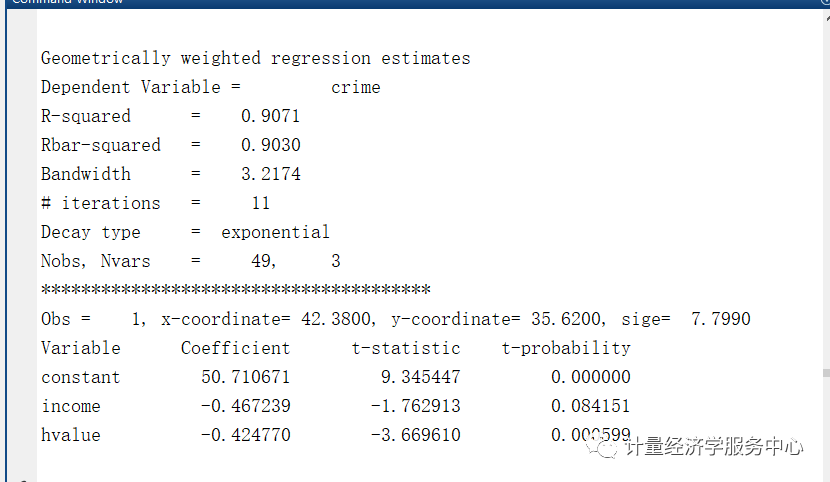
2-49空间单元参数估计结果不再展现
5
立方距离权重函数地理加权回归模型
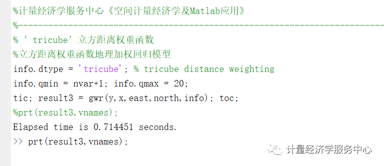
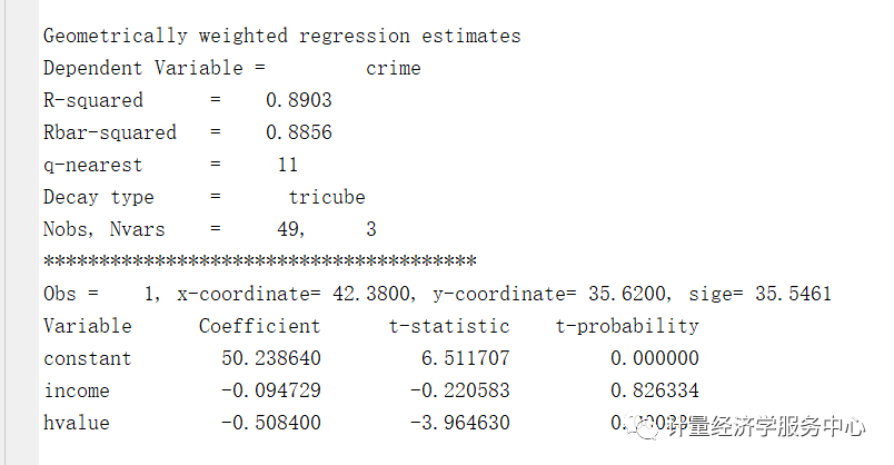
2-49空间单元参数估计结果不再展现
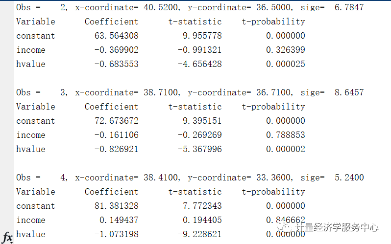
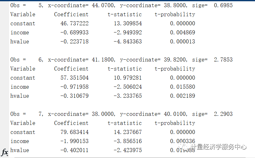
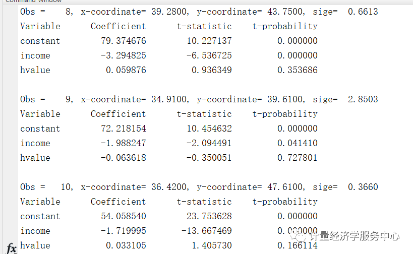
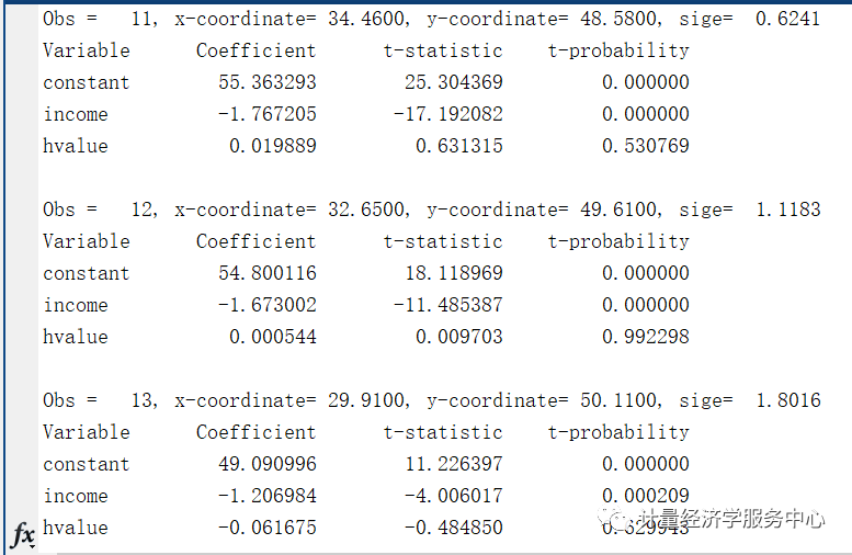
高斯距离权重函数地理加权回归模型1-49地理加权回归参数估计结果为:
%--------------------------------------------------------------------------%计量经济学服务中心《空间计量经济学及Matlab应用》%--------------------------------------------------------------------------Vname =VariableGeometrically weighted regression estimates Dependent Variable = crime R-squared = 0.9418 Rbar-squared = 0.9393 Bandwidth = 0.6518 # iterations = 17 Decay type = gaussian Nobs, Nvars = 49, 3 ***************************************Obs = 1, x-coordinate= 42.3800, y-coordinate= 35.6200, sige= 3.4125 Variable Coefficient t-statistic t-probability constant 51.197363 9.212794 0.000000 income -0.461038 -1.678857 0.099547 hvalue -0.434237 -3.693955 0.000556 Obs = 2, x-coordinate= 40.5200, y-coordinate= 36.5000, sige= 6.7847 Variable Coefficient t-statistic t-probability constant 63.564308 9.955778 0.000000 income -0.369902 -0.991321 0.326399 hvalue -0.683553 -4.656428 0.000025 Obs = 3, x-coordinate= 38.7100, y-coordinate= 36.7100, sige= 8.6457 Variable Coefficient t-statistic t-probability constant 72.673672 9.395151 0.000000 income -0.161106 -0.269269 0.788853 hvalue -0.826921 -5.367996 0.000002 Obs = 4, x-coordinate= 38.4100, y-coordinate= 33.3600, sige= 5.2400 Variable Coefficient t-statistic t-probability constant 81.381328 7.772343 0.000000 income 0.149437 0.194405 0.846662 hvalue -1.073198 -9.228621 0.000000 Obs = 5, x-coordinate= 44.0700, y-coordinate= 38.8000, sige= 0.6985 Variable Coefficient t-statistic t-probability constant 46.737222 13.309854 0.000000 income -0.689933 -2.949392 0.004869 hvalue -0.223718 -4.843363 0.000013 Obs = 6, x-coordinate= 41.1800, y-coordinate= 39.8200, sige= 2.7853 Variable Coefficient t-statistic t-probability constant 57.351504 10.979281 0.000000 income -0.971958 -2.506024 0.015580 hvalue -0.310679 -3.233765 0.002189 Obs = 7, x-coordinate= 38.0000, y-coordinate= 40.0100, sige= 2.2903 Variable Coefficient t-statistic t-probability constant 79.683414 14.237667 0.000000 income -1.990153 -3.856516 0.000336 hvalue -0.402011 -2.423975 0.019088 Obs = 8, x-coordinate= 39.2800, y-coordinate= 43.7500, sige= 0.6613 Variable Coefficient t-statistic t-probability constant 79.374676 10.227137 0.000000 income -3.294825 -6.536725 0.000000 hvalue 0.059876 0.936349 0.353686 Obs = 9, x-coordinate= 34.9100, y-coordinate= 39.6100, sige= 2.8503 Variable Coefficient t-statistic t-probability constant 72.218154 10.454632 0.000000 income -1.988247 -2.094491 0.041410 hvalue -0.063618 -0.350051 0.727801 Obs = 10, x-coordinate= 36.4200, y-coordinate= 47.6100, sige= 0.3660 Variable Coefficient t-statistic t-probability constant 54.058540 23.753628 0.000000 income -1.719995 -13.667469 0.000000 hvalue 0.033105 1.405730 0.166114 Obs = 11, x-coordinate= 34.4600, y-coordinate= 48.5800, sige= 0.6241 Variable Coefficient t-statistic t-probability constant 55.363293 25.304369 0.000000 income -1.767205 -17.192082 0.000000 hvalue 0.019889 0.631315 0.530769 Obs = 12, x-coordinate= 32.6500, y-coordinate= 49.6100, sige= 1.1183 Variable Coefficient t-statistic t-probability constant 54.800116 18.118969 0.000000 income -1.673002 -11.485387 0.000000 hvalue 0.000544 0.009703 0.992298 Obs = 13, x-coordinate= 29.9100, y-coordinate= 50.1100, sige= 1.8016 Variable Coefficient t-statistic t-probability constant 49.090996 11.226397 0.000000 income -1.206984 -4.006017 0.000209 hvalue -0.061675 -0.484850 0.629943 Obs = 14, x-coordinate= 27.8000, y-coordinate= 51.2400, sige= 1.1740 Variable Coefficient t-statistic t-probability constant 42.025898 8.693270 0.000000 income -1.049190 -2.353344 0.022662 hvalue 0.034076 0.168603 0.866803 Obs = 15, x-coordinate= 25.2400, y-coordinate= 50.8900, sige= 0.5074 Variable Coefficient t-statistic t-probability constant 42.023487 9.931361 0.000000 income -2.035189 -4.285382 0.000085 hvalue 0.541132 2.264220 0.028021 Obs = 16, x-coordinate= 27.9300, y-coordinate= 48.4400, sige= 1.8858 Variable Coefficient t-statistic t-probability constant 50.858338 11.840157 0.000000 income -0.970544 -2.036648 0.047108 hvalue -0.163386 -0.772214 0.443696 Obs = 17, x-coordinate= 31.9100, y-coordinate= 46.7300, sige= 1.9074 Variable Coefficient t-statistic t-probability constant 63.935965 23.149085 0.000000 income -1.851883 -8.000266 0.000000 hvalue -0.065988 -0.739344 0.463225 Obs = 18, x-coordinate= 35.9200, y-coordinate= 43.4400, sige= 1.0826 Variable Coefficient t-statistic t-probability constant 61.515865 14.934047 0.000000 income -1.892916 -5.019187 0.000007 hvalue 0.013062 0.157654 0.875377 Obs = 19, x-coordinate= 33.4600, y-coordinate= 43.3700, sige= 2.7225 Variable Coefficient t-statistic t-probability constant 65.413374 17.271159 0.000000 income -2.860764 -4.125718 0.000143 hvalue 0.275876 1.222495 0.227368 Obs = 20, x-coordinate= 33.1400, y-coordinate= 41.1300, sige= 5.0673 Variable Coefficient t-statistic t-probability constant 66.620907 8.186391 0.000000 income -1.619154 -1.246106 0.218651 hvalue -0.110761 -0.311593 0.756672 Obs = 21, x-coordinate= 31.6100, y-coordinate= 43.9500, sige= 2.6677 Variable Coefficient t-statistic t-probability constant 68.176378 23.711500 0.000000 income -3.351877 -5.596394 0.000001 hvalue 0.449873 2.009607 0.049996 Obs = 22, x-coordinate= 30.4000, y-coordinate= 44.1000, sige= 2.6080 Variable Coefficient t-statistic t-probability constant 68.744965 23.673393 0.000000 income -3.282837 -5.969185 0.000000 hvalue 0.438989 2.053138 0.045418 Obs = 23, x-coordinate= 29.1800, y-coordinate= 43.7000, sige= 2.8861 Variable Coefficient t-statistic t-probability constant 69.068145 17.943117 0.000000 income -3.326136 -5.847206 0.000000 hvalue 0.468812 1.914810 0.061364 Obs = 24, x-coordinate= 28.7800, y-coordinate= 41.0400, sige= 8.1087 Variable Coefficient t-statistic t-probability constant 77.271200 7.416531 0.000000 income -3.000189 -3.431018 0.001230 hvalue 0.167212 0.398976 0.691645 Obs = 25, x-coordinate= 27.3100, y-coordinate= 43.2300, sige= 4.0434 Variable Coefficient t-statistic t-probability constant 67.368725 9.525528 0.000000 income -3.069044 -3.468780 0.001099 hvalue 0.363366 0.754567 0.454120 Obs = 26, x-coordinate= 24.9600, y-coordinate= 42.6700, sige= 2.5678 Variable Coefficient t-statistic t-probability constant 61.306231 5.851086 0.000000 income 0.006368 0.004423 0.996489 hvalue -1.071954 -1.162870 0.250514 Obs = 27, x-coordinate= 25.9000, y-coordinate= 41.2100, sige= 6.2344 Variable Coefficient t-statistic t-probability constant 59.819535 4.913992 0.000010 income -1.697764 -1.212751 0.231040 hvalue -0.138505 -0.170688 0.865172 Obs = 28, x-coordinate= 25.8500, y-coordinate= 39.3200, sige= 5.2496 Variable Coefficient t-statistic t-probability constant 45.265068 2.954417 0.004803 income -2.135825 -1.284057 0.205161 hvalue 0.591982 0.883602 0.381226 Obs = 29, x-coordinate= 27.4900, y-coordinate= 41.0900, sige= 8.3927 Variable Coefficient t-statistic t-probability constant 72.899979 6.290465 0.000000 income -3.258441 -2.970188 0.004599 hvalue 0.307426 0.555503 0.581078 Obs = 30, x-coordinate= 28.8200, y-coordinate= 38.3200, sige= 6.0199 Variable Coefficient t-statistic t-probability constant 80.285094 7.449344 0.000000 income -0.676605 -0.717337 0.476572 hvalue -0.618717 -2.097025 0.041175 Obs = 31, x-coordinate= 30.9000, y-coordinate= 41.3100, sige= 5.9421 Variable Coefficient t-statistic t-probability constant 68.118651 7.883805 0.000000 income -1.803631 -2.133632 0.037905 hvalue 0.059481 0.178766 0.858859 Obs = 32, x-coordinate= 32.8800, y-coordinate= 39.3600, sige= 4.5678 Variable Coefficient t-statistic t-probability constant 58.637810 7.764366 0.000000 income 0.495270 0.487439 0.628121 hvalue -0.388646 -1.896549 0.063791 Obs = 33, x-coordinate= 30.6400, y-coordinate= 39.7200, sige= 5.1218 Variable Coefficient t-statistic t-probability constant 70.568456 9.798923 0.000000 income -0.218856 -0.335471 0.738702 hvalue -0.448133 -1.933095 0.059014 Obs = 34, x-coordinate= 30.3500, y-coordinate= 38.2900, sige= 3.1096 Variable Coefficient t-statistic t-probability constant 80.030552 12.784499 0.000000 income 0.036213 0.068159 0.945936 hvalue -0.786849 -5.179351 0.000004 Obs = 35, x-coordinate= 32.0900, y-coordinate= 36.6000, sige= 3.5543 Variable Coefficient t-statistic t-probability constant 63.967857 8.009308 0.000000 income 0.337987 0.382854 0.703484 hvalue -0.492099 -3.556112 0.000846 Obs = 36, x-coordinate= 34.0800, y-coordinate= 37.6000, sige= 2.7764 Variable Coefficient t-statistic t-probability constant 67.746908 11.590897 0.000000 income -0.755463 -0.934476 0.354641 hvalue -0.243619 -2.063643 0.044369 Obs = 37, x-coordinate= 36.1200, y-coordinate= 37.1300, sige= 5.2909 Variable Coefficient t-statistic t-probability constant 65.979447 8.493093 0.000000 income -0.082415 -0.089905 0.928729 hvalue -0.420816 -3.386697 0.001402 Obs = 38, x-coordinate= 36.3000, y-coordinate= 37.8500, sige= 4.1933 Variable Coefficient t-statistic t-probability constant 70.241135 9.853816 0.000000 income -0.851484 -1.007494 0.318647 hvalue -0.331039 -2.669386 0.010278 Obs = 39, x-coordinate= 36.4000, y-coordinate= 35.9500, sige= 7.5290 Variable Coefficient t-statistic t-probability constant 60.058183 6.254403 0.000000 income 1.346573 1.335110 0.188010 hvalue -0.676333 -5.334379 0.000002 Obs = 40, x-coordinate= 35.6000, y-coordinate= 35.7200, sige= 6.1315 Variable Coefficient t-statistic t-probability constant 59.441973 6.623725 0.000000 income 1.197840 1.197762 0.236772 hvalue -0.582346 -4.668150 0.000024 Obs = 41, x-coordinate= 34.6600, y-coordinate= 35.7600, sige= 4.4315 Variable Coefficient t-statistic t-probability constant 64.924831 8.369141 0.000000 income 0.077997 0.082850 0.934308 hvalue -0.395195 -3.149189 0.002788 Obs = 42, x-coordinate= 33.9200, y-coordinate= 36.1500, sige= 2.7971 Variable Coefficient t-statistic t-probability constant 68.995022 11.150905 0.000000 income -0.721014 -0.903935 0.370452 hvalue -0.276558 -2.460420 0.017450 Obs = 43, x-coordinate= 30.4200, y-coordinate= 34.0800, sige= 1.6449 Variable Coefficient t-statistic t-probability constant 42.987174 3.069301 0.003493 income -0.130118 -0.085542 0.932179 hvalue -0.015665 -0.079318 0.937103 Obs = 44, x-coordinate= 28.2600, y-coordinate= 30.3200, sige= 1.5262 Variable Coefficient t-statistic t-probability constant 38.427625 7.366893 0.000000 income -0.618892 -1.442734 0.155458 hvalue -0.192297 -0.847771 0.400688 Obs = 45, x-coordinate= 29.8500, y-coordinate= 27.9400, sige= 1.2787 Variable Coefficient t-statistic t-probability constant 31.201319 5.045446 0.000007 income -0.603071 -1.601338 0.115730 hvalue -0.061387 -0.506869 0.614520 Obs = 46, x-coordinate= 28.2100, y-coordinate= 27.2700, sige= 1.5429 Variable Coefficient t-statistic t-probability constant 27.113505 4.535402 0.000037 income -0.413367 -1.327768 0.190407 hvalue -0.043317 -0.586370 0.560318 Obs = 47, x-coordinate= 26.6900, y-coordinate= 24.2500, sige= 0.5555 Variable Coefficient t-statistic t-probability constant 24.205091 3.701915 0.000542 income -0.278691 -0.853556 0.397505 hvalue -0.032273 -0.812649 0.420350 Obs = 48, x-coordinate= 25.7100, y-coordinate= 25.4700, sige= 0.6629 Variable Coefficient t-statistic t-probability constant 24.211353 4.173486 0.000122 income -0.271872 -0.991422 0.326350 hvalue -0.034801 -0.854272 0.397112 Obs = 49, x-coordinate= 26.5800, y-coordinate= 29.0200, sige= 1.4185 Variable Coefficient t-statistic t-probability constant 30.052990 5.675101 0.000001 income -0.431664 -1.644271 0.106522 hvalue -0.081504 -0.934733 0.354510