Terminology
multivariant: 多元
excerpt: v.摘抄, n.片段
deviation: n.偏差
the standard deviation of the variable: 变量的标准差(方差的算术平方根)
iteration: 迭代
converge: 收敛
Polynomial: 多项式
quadratic function: 二次函数
cubic function: 三次函数
Normal Equation: 正规方程
get some intuition about sth: 了解一下
intuition: n.直觉
hassle: n.麻烦
regularization: 正则化
Multivariate Linear Regression
Hypothesis
h θ ( x ) = θ 0 + θ 1 x 1 + θ 2 x 2 + . . . + θ n x n h_\theta(x)=\theta_0+\theta_1x_1+\theta_2x_2+...+\theta_nx_nhθ(x)=θ0+θ1x1+θ2x2+...+θnxn
For convenience of notation, define x0=1.
x = [ x 0 x 1 x 2 ⋮ x n ] ∈ R n + 1 x= \left[ \begin{matrix} x_0 \\ x_1 \\ x_2 \\ \vdots \\ x_n \end{matrix} \right] \in \mathbb{R}^{n+1}x=⎣⎢⎢⎢⎢⎢⎡x0x1x2⋮xn⎦⎥⎥⎥⎥⎥⎤∈Rn+1
θ = [ θ 0 θ 1 θ 2 ⋮ θ n ] ∈ R n + 1 \theta= \left[ \begin{matrix} \theta_0 \\ \theta_1 \\ \theta_2 \\ \vdots \\ \theta_n \end{matrix} \right] \in \mathbb{R}^{n+1}θ=⎣⎢⎢⎢⎢⎢⎡θ0θ1θ2⋮θn⎦⎥⎥⎥⎥⎥⎤∈Rn+1
Then hypothesis can be written as:
h θ ( x ) = [ θ 0 θ 1 ⋯ θ n ] [ x 0 x 1 ⋮ x n ] = θ T x h_\theta(x)= \left[\begin{matrix} \theta_0 &\theta_1 &\cdots &\theta_n \end{matrix}\right] \left[\begin{matrix} x_0 \\ x_1 \\ \vdots \\ x_n \end{matrix}\right]= \theta^{T}xhθ(x)=[θ0θ1⋯θn]⎣⎢⎢⎢⎡x0x1⋮xn⎦⎥⎥⎥⎤=θTx
Gradient descent for multiple variables

New algorithm(n>=1):
Gradient Descent in Practice I - Feature Scaling
Feature Scaling
Idea: Make sure features are on a similar scale.
Target: Get every feature into approximately a -1 ≤xi≤ 1 range.
0<=x1<=3 (Y)
-2<=x2<=0.5 (Y)
-100<=x3<=100 (N)
-0.0001<=x4<=0.0001 (N)

0<=x1<=1, 0<=x2<=1
Accepted: -3 to 3, -1/3 to 1/3
Mean Normalization
Idea: Replace xi with xi- ui to make features have approximately zero mean(Do not apply to x0= 1).
x i : = x i − μ i s i x_i:=\frac{x_i-\mu_i}{s_i}xi:=sixi−μi
μi : the average of all the values for feature (i)
si : the range of values (max - min), or the standard deviation.
(测试用range,编程用标准差)

Gradient Descent in Practice II - Learning Rate
Making sure gradient descent is working correctly.
The job of gradient descent is to find the value of theta for you that hopefully minimizes the cost function J(θ).
plot the J(θ) as a function of the number of iterations can help to figure out what’s going on.

Automatic convergence test: However in practice it’s difficult to choose this threshold value.

It has been proven that if learning rate α is sufficiently small, then J(θ) will decrease on every iteration.

Summary:
- lf α is too small: slow convergence.
- lf α is too large: J(θ) may not decrease on every iteration; may not converge.
To choose α, try: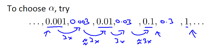
Features and Polynomial Regression
We can improve our features and the form of our hypothesis function in a couple different ways.
We can combine multiple features into one. For example, we can combine x1 and x2 into a new feature x3 by taking x1*x2.

Polynomial Regression
Using the machinery of multivariant linear regression, we can do this with a pretty simple modification to our algorithm.

Attention: Size should be applied feature scaling.
多项式回归允许你使用线性回归的机制来拟合非常复杂、甚至非线性的函数。
Choice of features
![[外链图片转存失败,源站可能有防盗链机制,建议将图片保存下来直接上传(img-wOcoPIZS-1650255003700)(G:\AI学习\ML\Week2.assets\image-20220417214936449.png)]](https://img-blog.csdnimg.cn/db36c63d26db4c8f91651a59aa20c728.png?x-oss-process=image/watermark,type_d3F5LXplbmhlaQ,shadow_50,text_Q1NETiBARmlsYmVydOeahOamm-WtkA==,size_20,color_FFFFFF,t_70,g_se,x_16)
Computing Parameters Analytically
Normal Equation
Normal Equation may give us a much better way to solve for the optimal value of the parameters θ.
In contrast to Gradient Descent, the normal equation would give us a method to solve for θ analytically, so that rather than needing to run this iterative algorithm, we can instead just solve for the optimal value for theta all at one go, so that in basically one step you get to the optimal value right there.
θ ∈ R n + 1 J ( θ 0 , θ 1 ) = 1 2 m ∑ i = 1 m ( y ^ i − y i ) 2 = 1 2 m ∑ i = 1 m ( h θ ( x i ) − y i ) 2 ∂ ∂ θ j J ( θ ) = . . . = 0 ( f o r e v e r y j ) \theta\in\mathbb{R}^{n+1} \\ J(θ_0,θ_1)= \frac{1}{2m} \sum_{i=1}^{m}({\hat{y}_i-y_i})^2= \frac{1}{2m}\sum_{i=1}^{m}(h_\theta(x_i)-y_i)^2 \\ \frac{\partial}{\partial\theta_j}J(\theta)=...=0(for~every~j)θ∈Rn+1J(θ0,θ1)=2m1i=1∑m(y^i−yi)2=2m1i=1∑m(hθ(xi)−yi)2∂θj∂J(θ)=...=0(for every j)
Solve for θ0, θ1, … , θn

θ = ( X T X ) − 1 X T y \textcolor{#FF0000}{\theta=(X^TX)^{-1}X^Ty}θ=(XTX)−1XTy
勘误:设计矩阵 X(在幻灯片的右下角)应该有元素x,下标为1,上标从1到m不等,因为对于所有m个训练集,只有2个特征x0和x1。
There is no need to do feature scaling with the normal equation.

With the normal equation, computing the inversion has complexity
O ( n 3 ) \mathcal{O}(n^3)O(n3)
So if we have a very large number of features, the normal equation will be slow. In practice, when n exceeds 10,000 it might be a good time to go from a normal solution to an iterative process.
Normal Equation Non-invertibility
What if XTX is non-invertible?(singular/degenerate)
If XTX is noninvertible, the common causes might be having :
Redundant features, where two features are very closely related (i.e. they are linearly dependent)
E.g. x1=size in feet2
x2=size in m2
Too many features (e.g. m ≤ n). In this case, delete some features or use regularization.
References
Coursera吴恩达机器学习编程作业下载及提交指南(Matlab 桌面版)
编程作业参考:
Coursera吴恩达机器学习课程 总结笔记及作业代码——第1,2周