
点击关注,桓峰基因
桓峰基因
生物信息分析,SCI文章撰写及生物信息基础知识学习:R语言学习,perl基础编程,linux系统命令,Python遇见更好的你
132篇原创内容
公众号
桓峰基因公众号推出基于R语言绘图教程并配有视频在线教程,目前整理出来的教程目录如下:
FigDraw 1. SCI 文章的灵魂 之 简约优雅的图表配色
FigDraw 2. SCI 文章绘图必备 R 语言基础
FigDraw 3. SCI 文章绘图必备 R 数据转换
FigDraw 4. SCI 文章绘图之散点图 (Scatter)
FigDraw 5. SCI 文章绘图之柱状图 (Barplot)
FigDraw 6. SCI 文章绘图之箱线图 (Boxplot)
FigDraw 7. SCI 文章绘图之折线图 (Lineplot)
FigDraw 8. SCI 文章绘图之饼图 (Pieplot)
FigDraw 9. SCI 文章绘图之韦恩图 (Vennplot)
FigDraw 10. SCI 文章绘图之直方图 (HistogramPlot)
FigDraw 11. SCI 文章绘图之小提琴图 (ViolinPlot)
FigDraw 12. SCI 文章绘图之相关性矩阵图(Correlation Matrix)
FigDraw 13. SCI 文章绘图之桑葚图及文章复现(Sankey)
FigDraw 14. SCI 文章绘图之和弦图及文章复现(Chord Diagram)
FigDraw 15. SCI 文章绘图之多组学圈图(OmicCircos)
前言
circos可以作为数据展示的一种手段,主要用于基因组数据的可视化,比如甲基化,组蛋白修饰,snp,indel,sv,以及常见的基因表达水平的展示,一般的circos都是基于perl语言的,数量繁多的配置文件总是很难按照我们想要的方式展示最终结果。而在R中也存在一些绘制circos的包,这期中主要介绍一下OmicCircos这个包的使用方法,做出来的circos图实属高大上,您不确定在自己的文章中来一个这样的图嘛?

软件安装
if (!require(OmicCircos)) BiocManager::install("OmicCircos")
library(OmicCircos)
options(stringsAsFactors = FALSE)
数据读取
首先导入自带数据进行测试,包括基因表达,cnv等数据。
data("TCGA.PAM50_genefu_hg18")
head(TCGA.PAM50_genefu_hg18)
##   chr        po  Gene     Basal        Her2       LumA        LumB      Normal
## 1   1 212873846 CENPF 0.4829763 -0.02926616 -0.5437402  0.27822856 -0.07058307
## 2   1 120072157 PHGDH 0.6345189 -0.18662586 -0.3986822 -1.03013932  0.66043775
## 3   1  43599336 CDC20 0.3996952  0.00835552 -0.4690440 -0.07041247 -0.04550481
## 4   1  44992051 KIF2C 0.2035726 -0.16510205 -0.5053947 -0.18289071 -0.39001448
## 5   1 161575262  NUF2 0.4724002 -0.02381921 -0.7125208  0.58962688 -0.37053337
## 6   1 200572562 UBE2T 0.3899089  0.28453681 -0.5392594  0.73895213 -0.95238101
data("TCGA.BC.fus")
head(TCGA.BC.fus)
##   chr1      po1    gene1 chr2       po2    gene2             name
## 1    2 63456333    WDPCP   10  37493749 ANKRD30A TCGA-BH-A18M-01A
## 2   18 14563374   PARD6G   21  14995400    POTED TCGA-BH-A1ET-01A
## 3   10 37521495 ANKRD30A    3  49282645   CCDC36 TCGA-BH-A1ET-01A
## 4   10 37521495 ANKRD30A    7 100177212    LRCH4 TCGA-BH-A1EU-01A
## 5   18 18539803    ROCK1   18    112551   PARD6G TCGA-BH-A1EW-11B
## 6   12  4618159  C12orf4   18   1514414   PARD6G TCGA-C8-A12Q-01A
data("TCGA.BC.cnv.2k.60")
head(TCGA.BC.cnv.2k.60)
##     chr        po     NAME TCGA.A1.A0SK.01A TCGA.A1.A0SO.01A TCGA.A2.A04W.01A
## 282  10 122272906 PPAPDC1A           -0.305            0.800            0.011
## 363  15  46973079     SHC4           -0.567           -0.813           -0.177
## 456  19  63014177   ZNF552            0.163            0.907            0.397
## 15    1  67590403  IL12RB2            0.098            0.347            0.165
## 381  16   8750130     ABAT           -0.634            0.478           -0.003
## 238   8  87486702     WWP1            1.035            0.340           -0.019
data("TCGA.BC.gene.exp.2k.60")
head(TCGA.BC.gene.exp.2k.60)
##     chr        po     NAME TCGA.A1.A0SK.01A TCGA.A1.A0SO.01A TCGA.A2.A04W.01A
## 282  10 122272906 PPAPDC1A           -0.809            0.224            1.639
## 363  15  46973079     SHC4           -0.704            3.656            1.631
## 456  19  63014177   ZNF552           -3.116            0.417            0.240
## 15    1  67590403  IL12RB2            3.420            4.054           -0.141
## 381  16   8750130     ABAT           -3.165           -1.880           -0.981
## 238   8  87486702     WWP1           -1.713           -2.314           -1.345
data("TCGA.BC.sample60")
head(TCGA.BC.sample60)
##             sample type
## 1 TCGA.A2.A0ET.01A LumA
## 2 TCGA.A8.A06Y.01A LumA
## 3 TCGA.A8.A083.01A LumA
## 4 TCGA.AN.A0FZ.01A LumA
## 5 TCGA.AO.A125.01A LumA
## 6 TCGA.AO.A12H.01A LumA
data("TCGA.BC_Her2_cnv_exp")
head(TCGA.BC_Her2_cnv_exp)
##     chr        po    gene t.value    Pvalue Bonferroni   FDR
## 282   3 127177852  ROPN1B   0.826 0.4240000          1 0.838
## 363   3 125181729   ROPN1   0.482 0.6380000          1 0.922
## 456   1  45566032    HPDL  -0.147 0.8860000          1 0.980
## 15   18  31986260    ELP2   4.310 0.0008467          1 0.068
## 381   7  93880144  COL1A2  -0.409 0.6890000          1 0.936
## 238   1 148948573 HORMAD1   1.017 0.3280000          1 0.783
参数说明
draw circular Description This is the main function of OmicCircos to draw circular plots. Usage circos(mapping=mapping, xc=400, yc=400, R=400, W=W, cir=“”, type=“n”, col.v=3, B=FALSE, print.chr.lab=TRUE, col.bar=FALSE, col.bar.po = “topleft”,
cluster=FALSE, order=NULL, scale=FALSE, cutoff = “n”, zoom=“”, cex=1, lwd=1, col=rainbow(10, alpha=0.8)[7], side=“”)
需要注意的是,omicCircos是使用type函数来指定不同图形的展示方式的,而type可以指定的图片形式包括以下几种:
“chr”:染色体或片段的绘图
“chr2”:染色体或部分基因组片段图
“heatmap”:热图
“heatmap2”:基因组坐标的heatmaps
“hightlight.link”:用于缩放的链接线
“hl”:突出显示
“label”:基因标签或文本注释
“label2”:具有相同圆周坐标的基因标签或文本注释
“link.pg”:基于贝塞尔曲线的链接多边形
“link”:基于贝塞尔曲线的链接线
“link2”:具有较小染色体内弧的链接线
“l”:折线
“ls”:阶梯状线图
“lh”:水平线
“ml”:多折线
“ml2”:多水平线
“ml3”:多阶梯状线图
“box”:箱线图
“hist”:多个样本的直方图
“ms”:多个样本的点图(类似箱线图)
“h”:柱状图
“s”:点图
“b”:条形图
“quant75”:75%分位数线
“quant90”:90%分位数线
“ss”:与数值成比例的点
“sv”:与方差成比例的点
“s.sd”:与标准偏差成比例的点
“ci95”:95%置信区间线
“b2”:条形图(双向)
“b3”:相同高度的条形图
“s2”:固定半径的点
“arc”:半径可变的弧(表示基因片段)
“arc2”:具有固定半径的弧
实例解析
在使用OmicCircos绘制circos图之前,我们首先也需要准备配置文件,比如染色体长度信息,染色体定位信息等等,如果还有snp,甲基化等信息也可以一并展示,在OmicCircos中主要使用circos函数来绘制circos图形。
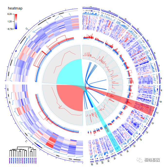
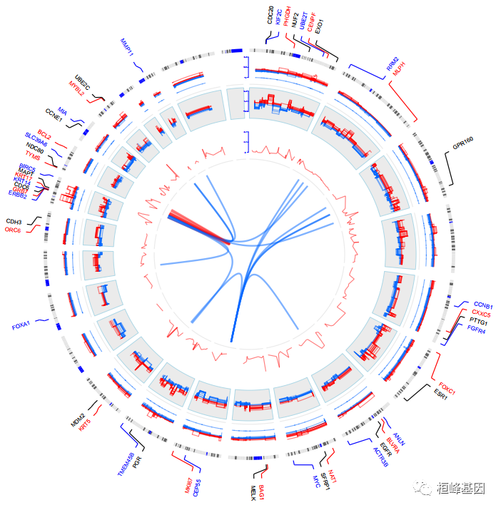
1. OmicCircos4vignette10
我们选择该软件包里面带有的第10个教程绘制circos图。这里就不多解释直接上代码,自行套用即可,这种图形都需要耐心仔细调图,非常耗时间。
#cnv的p值进行log10转化
pvalue <- -1 * log10(TCGA.BC_Her2_cnv_exp[,5]);
pvalue <- cbind(TCGA.BC_Her2_cnv_exp[,c(1:3)], pvalue);

#筛选Her2亚型
Her2.i <- which(TCGA.BC.sample60[,2] == "Her2");
Her2.n <- TCGA.BC.sample60[Her2.i,1];
Her2.j <- which(colnames(TCGA.BC.cnv.2k.60) %in% Her2.n);

#筛选Her2亚型患者cnv信息
cnv <- TCGA.BC.cnv.2k.60[,c(1:3,Her2.j)];
cnv.m <- cnv[,c(4:ncol(cnv))];
cnv.m[cnv.m >  2] <- 2;
cnv.m[cnv.m < -2] <- -2;
cnv <- cbind(cnv[,1:3], cnv.m);

#筛选Her2亚型患者的基因表达信息
Her2.j   <- which(colnames(TCGA.BC.gene.exp.2k.60) %in% Her2.n);
gene.exp <- TCGA.BC.gene.exp.2k.60[,c(1:3,Her2.j)];

#设定颜色
colors <- rainbow(10, alpha=0.5);

#画图,首先建立一个空白图层
pdf("OmicCircos4vignette10.pdf", 8,8);
par(mar=c(2, 2, 2, 2));
plot(c(1,800), c(1,800), type="n", axes=FALSE, xlab="", ylab="", main="");


#选择需要放大的坐标
zoom <- c(1, 22, 939245.5, 154143883, 0, 180);

#开始画图
circos(R=400, cir="hg18", W=4,   type="chr", print.chr.lab=TRUE, scale=TRUE, zoom=zoom);#最外层染色体信息
circos(R=300, cir="hg18", W=100, mapping=gene.exp, col.v=4,  type="heatmap2", cluster=TRUE, col.bar=TRUE, lwd=0.01, zoom=zoom);#次外层基因表达信息
circos(R=220, cir="hg18", W=80,  mapping=cnv,      col.v=4,   type="ml3", B=FALSE, lwd=1, cutoff=0, zoom=zoom);#第三层cnv信息
circos(R=140, cir="hg18", W=80,  mapping=pvalue,   col.v=4,    type="l",   B=TRUE, lwd=1, col=colors[1], zoom=zoom);#第四层p值曲线
circos(R=130, cir="hg18", W=10,  mapping=TCGA.BC.fus, type="link", lwd=2, zoom=zoom);#基因共表达连线


## 局部放大操作
the.col1=rainbow(10, alpha=0.5)[1];
highlight <- c(140, 400, 11, 282412.5, 11, 133770314.5, the.col1, the.col1);
circos(R=110, cir="hg18", W=40, mapping=highlight, type="hl", lwd=2, zoom=zoom);
the.col2=rainbow(10, alpha=0.5)[6];
highlight <- c(140, 400, 17, 739525, 17, 78385909, the.col2, the.col2);
circos(R=110, cir="hg18", W=40, mapping=highlight, type="hl", lwd=2, zoom=zoom);

## highlight link
highlight.link1 <- c(400, 400, 140, 376.8544, 384.0021, 450, 540.5);
circos(cir="hg18", mapping=highlight.link1, type="highlight.link", col=the.col1, lwd=1);
highlight.link2 <- c(400, 400, 140, 419.1154, 423.3032, 543, 627);
circos(cir="hg18", mapping=highlight.link2, type="highlight.link", col=the.col2, lwd=1);

## zoom in chromosome 11
zoom <- c(11, 11, 282412.5, 133770314.5, 180, 270);
circos(R=400, cir="hg18", W=4,   type="chr", print.chr.lab=TRUE, scale=TRUE, zoom=zoom);
circos(R=300, cir="hg18", W=100, mapping=gene.exp, col.v=4,  type="heatmap2", cluster=TRUE, lwd=0.01, zoom=zoom);
circos(R=220, cir="hg18", W=80,  mapping=cnv,      col.v=4,   type="ml3", B=FALSE, lwd=1, cutoff=0, zoom=zoom);
circos(R=140, cir="hg18", W=80,  mapping=pvalue,   col.v=4,    type="l",   B=TRUE, lwd=1, col=colors[1], zoom=zoom);

## zoom in chromosome 17
zoom <- c(17, 17, 739525, 78385909, 274, 356);
circos(R=400, cir="hg18", W=4,   type="chr", print.chr.lab=TRUE, scale=TRUE, zoom=zoom);
circos(R=300, cir="hg18", W=100, mapping=gene.exp, col.v=4,  type="heatmap2", cluster=TRUE, lwd=0.01, zoom=zoom);
circos(R=220, cir="hg18", W=80,  mapping=cnv,      col.v=4,   type="ml3", B=FALSE, lwd=1, cutoff=0, zoom=zoom);
circos(R=140, cir="hg18", W=80,  mapping=pvalue,   col.v=4,    type="l",   B=TRUE, lwd=1, col=colors[1], zoom=zoom);
dev.off()
## png
##   2
2. OmicCircos4vignette1
# \tdemo(OmicCircos4vignette1) \t---- ~~~~~~~~~~~~~~~~~~~~
rm(list = ls())
library(OmicCircos)
options(stringsAsFactors = FALSE)
set.seed(1234)
## initial values for simulation data
seg.num <- 10
ind.num <- 20
seg.po <- c(20:50)
link.num <- 10
link.pg.num <- 4

## output simulation data
sim.out <- sim.circos(seg = seg.num, po = seg.po, ind = ind.num, link = link.num,
    link.pg = link.pg.num)
seg.f <- sim.out$seg.frame
seg.v <- sim.out$seg.mapping
link.v <- sim.out$seg.link
link.pg.v <- sim.out$seg.link.pg
seg.num <- length(unique(seg.f[, 1]))

## select segments
seg.name <- paste("chr", 1:seg.num, sep = "")
db <- segAnglePo(seg.f, seg = seg.name)
colors <- rainbow(seg.num, alpha = 0.5)
pdffile <- "OmicCircos4vignette1.pdf"
pdf(pdffile, 8, 8)
par(mar = c(2, 2, 2, 2))
plot(c(1, 800), c(1, 800), type = "n", axes = FALSE, xlab = "", ylab = "", main = "")
circos(R = 400, cir = db, type = "chr", col = colors, print.chr.lab = TRUE, W = 4,
    scale = TRUE)
circos(R = 360, cir = db, W = 40, mapping = seg.v, col.v = 3, type = "l", B = TRUE,
    col = colors[1], lwd = 2, scale = TRUE)
circos(R = 320, cir = db, W = 40, mapping = seg.v, col.v = 3, type = "ls", B = FALSE,
    col = colors[9], lwd = 2, scale = TRUE)
circos(R = 280, cir = db, W = 40, mapping = seg.v, col.v = 3, type = "lh", B = TRUE,
    col = colors[7], lwd = 2, scale = TRUE)
circos(R = 240, cir = db, W = 40, mapping = seg.v, col.v = 19, type = "ml", B = FALSE,
    col = colors, lwd = 2, scale = TRUE)
circos(R = 200, cir = db, W = 40, mapping = seg.v, col.v = 19, type = "ml2", B = TRUE,
    col = colors, lwd = 2)
circos(R = 160, cir = db, W = 40, mapping = seg.v, col.v = 19, type = "ml3", B = FALSE,
    cutoff = 5, lwd = 2)
circos(R = 150, cir = db, W = 40, mapping = link.v, type = "link", lwd = 2, col = colors[c(1,
    7)])
circos(R = 150, cir = db, W = 40, mapping = link.pg.v, type = "link.pg", lwd = 2,
    col = sample(colors, link.pg.num))
dev.off()
## png
##   2


## detach(package:OmicCircos, unload=TRUE)
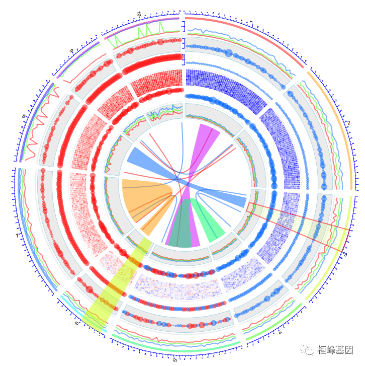
3. OmicCircos4vignette2
# \tdemo(OmicCircos4vignette2) \t---- ~~~~~~~~~~~~~~~~~~~~

rm(list = ls())
library(OmicCircos)
options(stringsAsFactors = FALSE)
set.seed(1234)

## initial values for simulation data
seg.num <- 10
ind.num <- 20
seg.po <- c(20:50)
link.num <- 10
link.pg.num <- 4

## output simulation data
sim.out <- sim.circos(seg = seg.num, po = seg.po, ind = ind.num, link = link.num,
    link.pg = link.pg.num)
seg.f <- sim.out$seg.frame
seg.v <- sim.out$seg.mapping
link.v <- sim.out$seg.link
link.pg.v <- sim.out$seg.link.pg
seg.num <- length(unique(seg.f[, 1]))

## select segments
seg.name <- paste("chr", 1:seg.num, sep = "")
db <- segAnglePo(seg.f, seg = seg.name)
colors <- rainbow(seg.num, alpha = 0.5)
pdffile <- "OmicCircos4vignette2.pdf"
pdf(pdffile, 8, 8)
par(mar = c(2, 2, 2, 2))
plot(c(1, 800), c(1, 800), type = "n", axes = FALSE, xlab = "", ylab = "", main = "")
circos(R = 400, type = "chr", cir = db, col = colors, print.chr.lab = TRUE, W = 4,
    scale = TRUE)
circos(R = 360, cir = db, W = 40, mapping = seg.v, col.v = 8, type = "box", B = TRUE,
    col = colors[1], lwd = 0.1, scale = TRUE)
circos(R = 320, cir = db, W = 40, mapping = seg.v, col.v = 8, type = "hist", B = TRUE,
    col = colors[3], lwd = 0.1, scale = TRUE)
circos(R = 280, cir = db, W = 40, mapping = seg.v, col.v = 8, type = "ms", B = TRUE,
    col = colors[7], lwd = 0.1, scale = TRUE)
circos(R = 240, cir = db, W = 40, mapping = seg.v, col.v = 3, type = "h", B = FALSE,
    col = colors[2], lwd = 0.1)
circos(R = 200, cir = db, W = 40, mapping = seg.v, col.v = 3, type = "s", B = TRUE,
    col = colors, lwd = 0.1)
circos(R = 160, cir = db, W = 40, mapping = seg.v, col.v = 3, type = "b", B = FALSE,
    col = colors, lwd = 0.1)
circos(R = 150, cir = db, W = 40, mapping = link.v, type = "link", lwd = 2, col = colors[c(1,
    7)])
circos(R = 150, cir = db, W = 40, mapping = link.pg.v, type = "link.pg", lwd = 2,
    col = sample(colors, link.pg.num))
dev.off()
## png
##   2

## detach(package:OmicCircos, unload=TRUE)

4. OmicCircos4vignette3
# demo(OmicCircos4vignette3) \t---- ~~~~~~~~~~~~~~~~~~~~

rm(list = ls())
library(OmicCircos)
options(stringsAsFactors = FALSE)
set.seed(1234)

## initial values for simulation data
seg.num <- 10
ind.num <- 20
seg.po <- c(20:50)
link.num <- 10
link.pg.num <- 4

## output simulation data
sim.out <- sim.circos(seg = seg.num, po = seg.po, ind = ind.num, link = link.num,
    link.pg = link.pg.num)
seg.f <- sim.out$seg.frame
seg.v <- sim.out$seg.mapping
link.v <- sim.out$seg.link
link.pg.v <- sim.out$seg.link.pg
seg.num <- length(unique(seg.f[, 1]))

## select segments
seg.name <- paste("chr", 1:seg.num, sep = "")
db <- segAnglePo(seg.f, seg = seg.name)
colors <- rainbow(seg.num, alpha = 0.5)
pdffile <- "OmicCircos4vignette3.pdf"
pdf(pdffile, 8, 8)
par(mar = c(2, 2, 2, 2))
plot(c(1, 800), c(1, 800), type = "n", axes = FALSE, xlab = "", ylab = "", main = "")
circos(R = 400, type = "chr", cir = db, col = colors, print.chr.lab = TRUE, W = 4,
    scale = TRUE)
circos(R = 360, cir = db, W = 40, mapping = seg.v, col.v = 8, type = "quant90", B = FALSE,
    col = colors, lwd = 2, scale = TRUE)
circos(R = 320, cir = db, W = 40, mapping = seg.v, col.v = 3, type = "sv", B = TRUE,
    col = colors[7], scale = TRUE)
circos(R = 280, cir = db, W = 40, mapping = seg.v, col.v = 3, type = "ss", B = FALSE,
    col = colors[3], scale = TRUE)
circos(R = 240, cir = db, W = 40, mapping = seg.v, col.v = 8, type = "heatmap", lwd = 3)
circos(R = 200, cir = db, W = 40, mapping = seg.v, col.v = 3, type = "s.sd", B = FALSE,
    col = colors[4])
circos(R = 160, cir = db, W = 40, mapping = seg.v, col.v = 3, type = "ci95", B = TRUE,
    col = colors[4], lwd = 2)
circos(R = 150, cir = db, W = 40, mapping = link.v, type = "link", lwd = 2, col = colors[c(1,
    7)])
circos(R = 150, cir = db, W = 40, mapping = link.pg.v, type = "link.pg", lwd = 2,
    col = sample(colors, link.pg.num))
the.col1 = rainbow(10, alpha = 0.5)[3]
highlight <- c(160, 410, 6, 2, 6, 10, the.col1, the.col1)
circos(R = 110, cir = db, W = 40, mapping = highlight, type = "hl", lwd = 1)
the.col1 = rainbow(10, alpha = 0.1)[3]
the.col2 = rainbow(10, alpha = 0.5)[1]
highlight <- c(160, 410, 3, 12, 3, 20, the.col1, the.col2)
circos(R = 110, cir = db, W = 40, mapping = highlight, type = "hl", lwd = 2)
dev.off()
## png
##   2


## detach(package:OmicCircos, unload=TRUE)
5. OmicCircos4vignette4
# \tdemo(OmicCircos4vignette4) \t---- ~~~~~~~~~~~~~~~~~~~~

rm(list = ls())
library(OmicCircos)
options(stringsAsFactors = FALSE)
set.seed(1234)
## load mm cytogenetic band data
data("UCSC.mm10.chr", package = "OmicCircos")
ref <- UCSC.mm10.chr
ref[, 1] <- gsub("chr", "", ref[, 1])

## initial values for simulation data
colors <- rainbow(10, alpha = 0.8)
lab.n <- 50
cnv.n <- 200
arc.n <- 30
fus.n <- 10

## make arc data
arc.d <- c()
for (i in1:arc.n) {
    chr <- sample(1:19, 1)
    chr.i <- which(ref[, 1] == chr)
    chr.arc <- ref[chr.i, ]
    arc.i <- sample(1:nrow(chr.arc), 2)
    arc.d <- rbind(arc.d, c(chr.arc[arc.i[1], c(1, 2)], chr.arc[arc.i[2], c(2, 4)]))
}

colnames(arc.d) <- c("chr", "start", "end", "value")

## make fusion data
fus.d <- c()

for (i in1:fus.n) {
    chr1 <- sample(1:19, 1)
    chr2 <- sample(1:19, 1)
    chr1.i <- which(ref[, 1] == chr1)
    chr2.i <- which(ref[, 1] == chr2)
    chr1.f <- ref[chr1.i, ]
    chr2.f <- ref[chr2.i, ]
    fus1.i <- sample(1:nrow(chr1.f), 1)
    fus2.i <- sample(1:nrow(chr2.f), 1)
    n1 <- paste0("geneA", i)
    n2 <- paste0("geneB", i)
    fus.d <- rbind(fus.d, c(chr1.f[fus1.i, c(1, 2)], n1, chr2.f[fus2.i, c(1, 2)],
        n2))
}

colnames(fus.d) <- c("chr1", "po1", "gene1", "chr2", "po2", "gene2")
cnv.i <- sample(1:nrow(ref), cnv.n)
vale <- rnorm(cnv.n)
cnv.d <- data.frame(ref[cnv.i, c(1, 2)], value = vale)
pdffile <- "OmicCircos4vignette4.pdf"
pdf(pdffile, 8, 8)
par(mar = c(2, 2, 2, 2))
plot(c(1, 800), c(1, 800), type = "n", axes = FALSE, xlab = "", ylab = "")
circos(R = 400, type = "chr", cir = "mm10", print.chr.lab = TRUE, W = 4, scale = TRUE)
circos(R = 340, cir = "mm10", W = 60, mapping = cnv.d, type = "b3", B = TRUE, col = colors[7])
circos(R = 340, cir = "mm10", W = 60, mapping = cnv.d, type = "s2", B = FALSE, col = colors[1],
    cex = 0.5)
circos(R = 280, cir = "mm10", W = 60, mapping = arc.d, type = "arc2", B = FALSE,
    col = colors, lwd = 10, cutoff = 0)
circos(R = 220, cir = "mm10", W = 60, mapping = cnv.d, col.v = 3, type = "b2", B = TRUE,
    cutoff = -0.2, col = colors[c(7, 9)], lwd = 2)
circos(R = 160, cir = "mm10", W = 60, mapping = arc.d, col.v = 4, type = "arc", B = FALSE,
    col = colors[c(1, 7)], lwd = 4, scale = TRUE)
circos(R = 150, cir = "mm10", W = 10, mapping = fus.d, type = "link", lwd = 2, col = colors[c(1,
    7, 9)])
dev.off()
## png
##   2

# detach(package:OmicCircos, unload=TRUE)
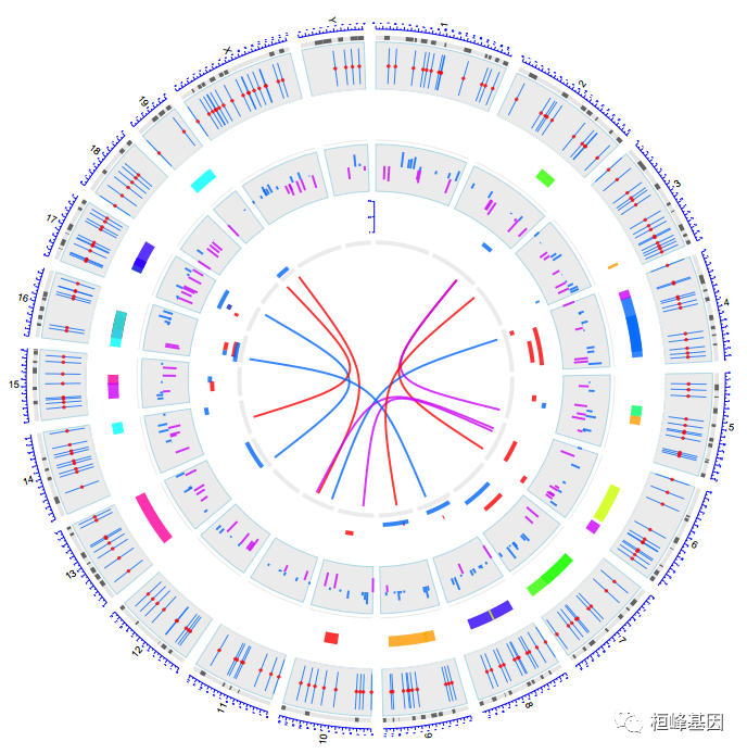
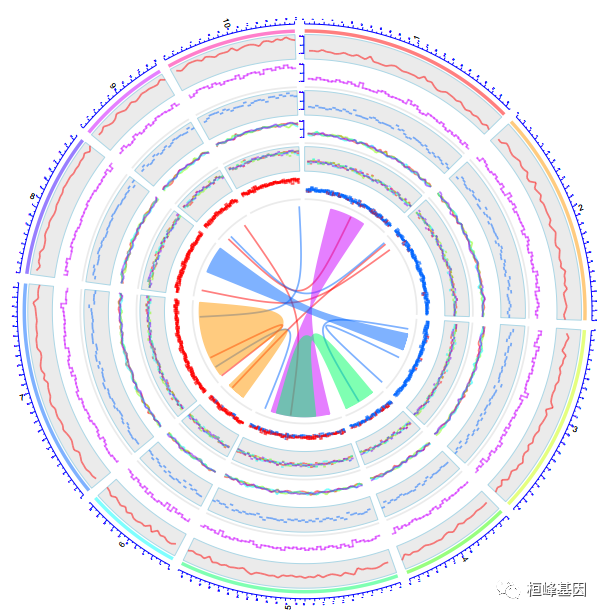
6. OmicCircos4vignette5
# \tdemo(OmicCircos4vignette5) \t---- ~~~~~~~~~~~~~~~~~~~~

rm(list = ls())
library(OmicCircos)
options(stringsAsFactors = FALSE)
set.seed(1234)
data("TCGA.PAM50_genefu_hg18")
data("TCGA.BC.fus")
data("TCGA.BC.cnv.2k.60")
data("TCGA.BC.gene.exp.2k.60")
data("TCGA.BC.sample60")
data("TCGA.BC_Her2_cnv_exp")
pvalue <- -1 * log10(TCGA.BC_Her2_cnv_exp[, 5])
pvalue <- cbind(TCGA.BC_Her2_cnv_exp[, c(1:3)], pvalue)
Her2.i <- which(TCGA.BC.sample60[, 2] == "Her2")
Her2.n <- TCGA.BC.sample60[Her2.i, 1]
Her2.j <- which(colnames(TCGA.BC.cnv.2k.60) %in% Her2.n)
cnv <- TCGA.BC.cnv.2k.60[, c(1:3, Her2.j)]
cnv.m <- cnv[, c(4:ncol(cnv))]
cnv.m[cnv.m <- 2] <- 2
cnv.m[cnv.m <- 2] <- -2
cnv <- cbind(cnv[, 1:3], cnv.m)
Her2.j <- which(colnames(TCGA.BC.gene.exp.2k.60) %in% Her2.n)
gene.exp <- TCGA.BC.gene.exp.2k.60[, c(1:3, Her2.j)]
colors <- rainbow(10, alpha = 0.5)
pdffile <- "OmicCircos4vignette5.pdf"
pdf(pdffile, 8, 8)
par(mar = c(2, 2, 2, 2))
plot(c(1, 800), c(1, 800), type = "n", axes = FALSE, xlab = "", ylab = "")
circos(R = 300, type = "chr", cir = "hg18", print.chr.lab = FALSE, W = 4)
circos(R = 310, cir = "hg18", W = 20, mapping = TCGA.PAM50_genefu_hg18, type = "label",
    side = "out", col = c("black", "blue", "red"), cex = 0.4)
circos(R = 250, cir = "hg18", W = 50, mapping = cnv, col.v = 4, type = "ml3", B = FALSE,
    col = colors[7], cutoff = 0, scale = TRUE)
circos(R = 200, cir = "hg18", W = 50, mapping = gene.exp, col.v = 4, type = "ml3",
    B = TRUE, col = colors[3], cutoff = 0, scale = TRUE)
circos(R = 140, cir = "hg18", W = 50, mapping = pvalue, col.v = 4, type = "l", B = FALSE,
    col = colors[1], scale = TRUE)

## set fusion gene colors
cols <- rep(colors[7], nrow(TCGA.BC.fus))
col.i <- which(TCGA.BC.fus[, 1] == TCGA.BC.fus[, 4])
cols[col.i] <- colors[1]
circos(R = 132, cir = "hg18", W = 50, mapping = TCGA.BC.fus, type = "link", col = cols,
    lwd = 2)
plot(c(1, 800), c(1, 800), type = "n", axes = FALSE, xlab = "", ylab = "")
circos(R = 300, type = "chr", cir = "hg18", col = TRUE, print.chr.lab = FALSE, W = 4)
circos(R = 290, cir = "hg18", W = 20, mapping = TCGA.PAM50_genefu_hg18, type = "label",
    side = "in", col = c("black", "blue"), cex = 0.4)
circos(R = 310, cir = "hg18", W = 50, mapping = cnv, col.v = 4, type = "ml3", B = TRUE,
    col = colors[7], cutoff = 0, scale = TRUE)
circos(R = 150, cir = "hg18", W = 50, mapping = gene.exp, col.v = 4, type = "ml3",
    B = TRUE, col = colors[3], cutoff = 0, scale = TRUE)
circos(R = 90, cir = "hg18", W = 50, mapping = pvalue, col.v = 4, type = "l", B = FALSE,
    col = colors[1], scale = TRUE)
circos(R = 82, cir = "hg18", W = 50, mapping = TCGA.BC.fus, type = "link", col = cols,
    lwd = 2)

dev.off()
## png
##   2

# detach(package:OmicCircos, unload=TRUE)
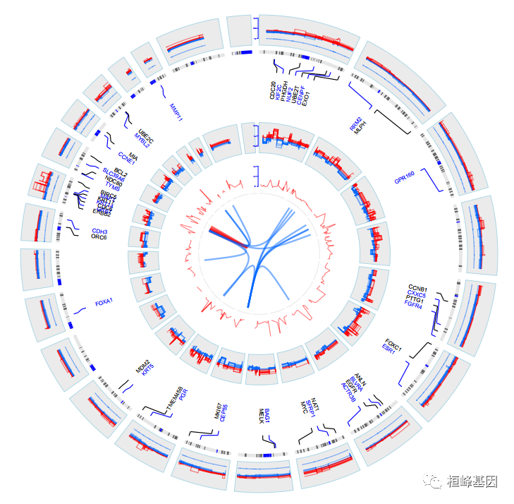
7. OmicCircos4vignette6
# \tdemo(OmicCircos4vignette6) \t---- ~~~~~~~~~~~~~~~~~~~~

rm(list = ls())
library(OmicCircos)
options(stringsAsFactors = FALSE)
data("TCGA.PAM50_genefu_hg18")
data("TCGA.BC.fus")
data("TCGA.BC.cnv.2k.60")
data("TCGA.BC.gene.exp.2k.60")
data("TCGA.BC.sample60")
data("TCGA.BC_Her2_cnv_exp")
pvalue <- -1 * log10(TCGA.BC_Her2_cnv_exp[, 5])
pvalue <- cbind(TCGA.BC_Her2_cnv_exp[, c(1:3)], pvalue)
Her2.i <- which(TCGA.BC.sample60[, 2] == "Her2")
Her2.n <- TCGA.BC.sample60[Her2.i, 1]
Her2.j <- which(colnames(TCGA.BC.cnv.2k.60) %in% Her2.n)
cnv <- TCGA.BC.cnv.2k.60[, c(1:3, Her2.j)]
cnv.m <- cnv[, c(4:ncol(cnv))]
cnv.m[cnv.m <- 2] <- 2
cnv.m[cnv.m <- 2] <- -2
cnv <- cbind(cnv[, 1:3], cnv.m)
Her2.j <- which(colnames(TCGA.BC.gene.exp.2k.60) %in% Her2.n)
gene.exp <- TCGA.BC.gene.exp.2k.60[, c(1:3, Her2.j)]
colors <- rainbow(10, alpha = 0.5)

pdf("OmicCircos4vignette6.pdf", 8, 8)
par(mar = c(2, 2, 2, 2))
plot(c(1, 800), c(1, 800), type = "n", axes = FALSE, xlab = "", ylab = "", main = "")
circos(R = 400, cir = "hg18", W = 4, type = "chr", print.chr.lab = TRUE, scale = TRUE)
circos(R = 300, cir = "hg18", W = 100, mapping = gene.exp, col.v = 4, type = "heatmap2",
    cluster = TRUE, col.bar = TRUE, lwd = 0.1, col = "blue")
circos(R = 220, cir = "hg18", W = 80, mapping = cnv, col.v = 4, type = "ml3", B = FALSE,
    lwd = 1, cutoff = 0)
circos(R = 140, cir = "hg18", W = 80, mapping = pvalue, col.v = 4, type = "l", B = TRUE,
    lwd = 1, col = colors[1])
cols <- rep(colors[7], nrow(TCGA.BC.fus))
col.i <- which(TCGA.BC.fus[, 1] == TCGA.BC.fus[, 4])
cols[col.i] <- colors[1]
circos(R = 130, cir = "hg18", W = 10, mapping = TCGA.BC.fus, type = "link2", lwd = 2,
    col = cols)
dev.off()
## png
##   2


# detach(package:OmicCircos, unload=TRUE)
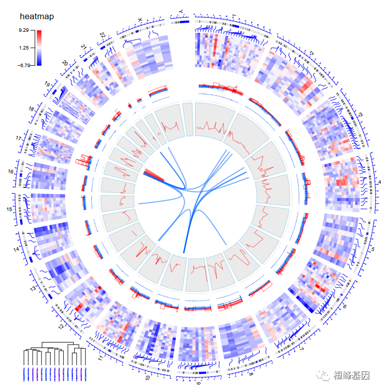
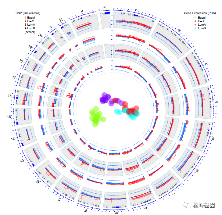
8. OmicCircos4vignette7
# \tdemo(OmicCircos4vignette7) \t---- ~~~~~~~~~~~~~~~~~~~~

rm(list = ls())
library(OmicCircos)
options(stringsAsFactors = FALSE)
data("TCGA.BC.fus")
data("TCGA.BC.cnv.2k.60")
data("TCGA.BC.gene.exp.2k.60")
data("TCGA.BC.sample60")

## gene expression data for PCA
exp.m <- TCGA.BC.gene.exp.2k.60[, c(4:ncol(TCGA.BC.gene.exp.2k.60))]
cnv <- TCGA.BC.cnv.2k.60

## PCA
type.n <- unique(TCGA.BC.sample60[, 2])
colors <- rainbow(length(type.n), alpha = 0.5)
pca.col <- rep(NA, nrow(TCGA.BC.sample60))

for (i in1:length(type.n)) {
    n <- type.n[i]
    n.i <- which(TCGA.BC.sample60[, 2] == n)
    n.n <- TCGA.BC.sample60[n.i, 1]
    g.i <- which(colnames(exp.m) %in% n.n)
    pca.col[g.i] <- colors[i]
}

exp.m <- na.omit(exp.m)
pca.out <- prcomp(t(exp.m), scale = TRUE)

## subtype cnv
cnv.i <- c()

for (i in1:length(type.n)) {
    n <- type.n[i]
    n.i <- which(TCGA.BC.sample60[, 2] == n)
    n.n <- TCGA.BC.sample60[n.i, 1]
    cnv.i <- which(colnames(cnv) %in% n.n)
}

## main
pdf("OmicCircos4vignette7.pdf", 8, 8)
par(mar = c(5, 5, 5, 5))
plot(pca.out$x[, 1] * 8, pca.out$x[, 2] * 8, pch = 19, col = pca.col, main = "",
    cex = 2, xlab = "PC1", ylab = "PC2", ylim = c(-200, 460), xlim = c(-200, 460))
legend(200, 0, c("Basal", "Her2", "LumA", "LumB"), pch = 19, col = colors[c(2, 4,
    1, 3)], cex = 1, title = "Gene Expression (PCA)", box.col = "white")
circos(xc = 260, yc = 260, R = 200, cir = "hg18", W = 4, type = "chr", print.chr.lab = TRUE)

R.v <- 160

for (i in1:length(type.n)) {
    n <- type.n[i]
    n.i <- which(TCGA.BC.sample60[, 2] == n)
    n.n <- TCGA.BC.sample60[n.i, 1]
    cnv.i <- which(colnames(cnv) %in% n.n)
    cnv.v <- cnv[, cnv.i]
    cnv.v[cnv.v <- 2] <- 2
    cnv.v[cnv.v <- 2] <- -2
    cnv.m <- cbind(cnv[, c(1:3)], cnv.v)
    if (i%%2 == 1) {
        circos(xc = 260, yc = 260, R = R.v, cir = "hg18", W = 30, mapping = cnv.m,
            col.v = 4, type = "ml3", B = TRUE, lwd = 0.5, cutoff = 0)
    } else {
        circos(xc = 260, yc = 260, R = R.v, cir = "hg18", W = 30, mapping = cnv.m,
            col.v = 4, type = "ml3", B = FALSE, lwd = 0.5, cutoff = 0)
    }

    R.v <- R.v - 30
}

legend(-140, 460, c("1 Basal", "2 Her2", "3 LumA", "4 LumB", "(center)"), cex = 1,
    title = "CNV (OmicCircos)", box.col = "white")

dev.off()
## png
##   2


## detach(package:OmicCircos, unload=TRUE)

9. OmicCircos4vignette8
# \tdemo(OmicCircos4vignette8) \t---- ~~~~~~~~~~~~~~~~~~~~

rm(list = ls())
library(OmicCircos)
options(stringsAsFactors = FALSE)
data("TCGA.BC.fus")
data("TCGA.BC.cnv.2k.60")
data("TCGA.BC.gene.exp.2k.60")
data("TCGA.BC.sample60")
## gene expression data for PCA
exp.m <- TCGA.BC.gene.exp.2k.60[, c(4:ncol(TCGA.BC.gene.exp.2k.60))]
cnv <- TCGA.BC.cnv.2k.60

## PCA
type.n <- unique(TCGA.BC.sample60[, 2])
colors <- rainbow(length(type.n), alpha = 0.5)
pca.col <- rep(NA, nrow(TCGA.BC.sample60))

for (i in1:length(type.n)) {
    n <- type.n[i]
    n.i <- which(TCGA.BC.sample60[, 2] == n)
    n.n <- TCGA.BC.sample60[n.i, 1]
    g.i <- which(colnames(exp.m) %in% n.n)
    pca.col[g.i] <- colors[i]
}

exp.m <- na.omit(exp.m)
pca.out <- prcomp(t(exp.m), scale = TRUE)

## subtype cnv
cnv.i <- c()

for (i in1:length(type.n)) {
    n <- type.n[i]
    n.i <- which(TCGA.BC.sample60[, 2] == n)
    n.n <- TCGA.BC.sample60[n.i, 1]
    cnv.i <- which(colnames(cnv) %in% n.n)
}

## main
pdf("OmicCircos4vignette8.pdf", 8, 8)
par(mar = c(5, 5, 5, 5))
plot(c(1, 800), c(1, 800), type = "n", axes = FALSE, xlab = "", ylab = "", main = "")
legend(680, 800, c("Basal", "Her2", "LumA", "LumB"), pch = 19, col = colors[c(2,
    4, 1, 3)], cex = 0.5, title = "Gene Expression (PCA)", box.col = "white")

legend(5, 800, c("1 Basal", "2 Her2", "3 LumA", "4 LumB", "(center)"), cex = 0.5,
    title = "CNV (OmicCircos)", box.col = "white")
circos(xc = 400, yc = 400, R = 390, cir = "hg18", W = 4, type = "chr", print.chr.lab = TRUE,
    scale = TRUE)

R.v <- 330

for (i in1:length(type.n)) {
    n <- type.n[i]
    n.i <- which(TCGA.BC.sample60[, 2] == n)
    n.n <- TCGA.BC.sample60[n.i, 1]
    cnv.i <- which(colnames(cnv) %in% n.n)
    cnv.v <- cnv[, cnv.i]
    cnv.v[cnv.v <- 2] <- 2
    cnv.v[cnv.v <- 2] <- -2
    cnv.m <- cbind(cnv[, c(1:3)], cnv.v)
    if (i%%2 == 1) {
        circos(xc = 400, yc = 400, R = R.v, cir = "hg18", W = 60, mapping = cnv.m,
            col.v = 4, type = "ml3", B = TRUE, lwd = 1, cutoff = 0, scale = TRUE)
    } else {
        circos(xc = 400, yc = 400, R = R.v, cir = "hg18", W = 60, mapping = cnv.m,
            col.v = 4, type = "ml3", B = FALSE, lwd = 1, cutoff = 0, scale = TRUE)
    }
    R.v <- R.v - 60
}

points(pca.out$x[, 1] * 6 + 410, pca.out$x[, 2] * 6 + 400, pch = 19, col = pca.col,
    cex = 2)

dev.off()
## png
##   2


## detach(package:OmicCircos, unload=TRUE)
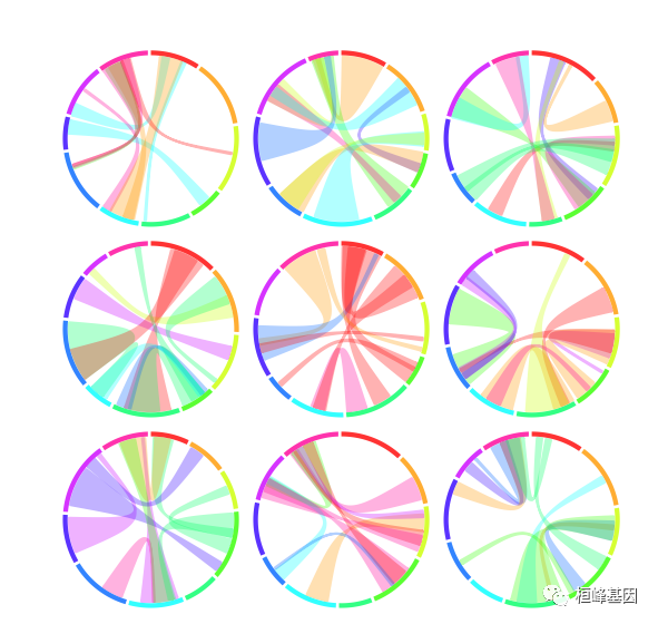
10. OmicCircos4vignette9
# \tdemo(OmicCircos4vignette9) \t---- ~~~~~~~~~~~~~~~~~~~~

rm(list = ls())
library(OmicCircos)
options(stringsAsFactors = FALSE)
perm_list <- function(n, r, v = 1:n) {
    if (r == 1)
        X <- matrix(v, n, 1) elseif (n == 1)
        X <- matrix(v, 1, r) else {
        X <- NULL
        for (i in1:n) {
            X <- rbind(X, cbind(v[i], perm_list(n - 1, r - 1, v[-i])))
        }
    }
    return(X)
}

## initial
seg.num <- 10

ind.num <- 20
seg.po <- c(20:50)
link.num <- 10
link.pg.num <- 10

## select segments
seg.name <- paste("chr", 1:seg.num, sep = "")
center <- c(200, 400, 600)
center.i <- perm_list(3, 2)

for (i in1:3) {
    center.i <- rbind(center.i, rep(i, 2))
}

colors <- rainbow(seg.num, alpha = 0.8)
color2 <- rainbow(10, alpha = 0.3)

pdffile <- "OmicCircos4vignette9.pdf"
pdf(pdffile, 8, 8)
par(mar = c(2, 2, 2, 2))
plot(c(1, 800), c(1, 800), type = "n", axes = FALSE, xlab = "", ylab = "", main = "")

for (i in1:nrow(center.i)) {
    xc <- center[center.i[i, 1]]
    yc <- center[center.i[i, 2]]
    sim.out <- sim.circos(seg = seg.num, po = seg.po, ind = ind.num, link = link.num,
        link.pg = link.pg.num)
    db <- segAnglePo(sim.out$seg.f, seg = seg.name)
    link.pg.v <- sim.out$seg.link.pg
    circos(xc = xc, yc = yc, R = 90, type = "chr", cir = db, col = colors, print.chr.lab = FALSE,
        W = 4)
    cols <- sample(color2, nrow(link.pg.v), replace = TRUE)
    circos(xc = xc, yc = yc, R = 86, cir = db, mapping = link.pg.v, type = "link.pg",
        lwd = 2, col = cols)

}

dev.off()
## png
##   2


## detach(package:OmicCircos, unload=TRUE)
软件包里面自带的demo,我这里都展示了一遍为了方便大家选择适合自己的图形,另外需要代码的将这期教程转发朋友圈,并配文“学生信,找桓峰基因,铸造成功的你!”
桓峰基因,铸造成功的您!
References:
- OmicCircos: an R package for simple and circular visualization of omics data. Cancer Inform. 2014 Jan 16;13:13-20. doi: 10.4137/CIN.S13495. eCollection 2014.