Programming Exercise 2: Logistic Regression

在本次练习中，你将实现逻辑回归并将其应用于两个不同的数据集。

在整个练习中，您将使用脚本ex2.m和ex2_reg.m。这些脚本设置了问题的数据集并调用了将要编写的函数

1 Logistic Regression

在本部分的练习中，您将建立一个Logistic回归模型来预测学生是否被大学录取，假设您是大学部门的管理员，并且您想根据每个申请人的入学机会来确定他们的入学机会。两次考试的结果。您拥有以前申请人的历史数据，可以用作逻辑回归的训练集。对于每个培训示例，您都有两次考试的申请人分数和录取决定。您的任务是建立一个分类模型，根据这两次考试的分数估算申请人的录取概率。此大纲和ex2.m中的框架代码将指导您完成本练习。

1.1 Visualizing the data

在开始实施任何学习算法之前，如果可能的话，最好可视化数据。在ex2.m的第一部分中，代码将加载数据并将其通过调用plotData.m函数显示在二维图上。您现在将在plotData.m中完成代码，以使其显示如图1所示的图形。轴是两个考试分数，正例和负例用不同的标记显示。

plotData.m

function plotData(X, y)
%PLOTDATA Plots the data points X and y into a new figure 
%   PLOTDATA(x,y) plots the data points with + for the positive examples
%   and o for the negative examples. X is assumed to be a Mx2 matrix.

% Create New Figure
figure; hold on;

% ====================== YOUR CODE HERE ======================
% Instructions: Plot the positive and negative examples on a
%               2D plot, using the option 'k+' for the positive
%               examples and 'ko' for the negative examples.
%

X1=X(:,1);X2=X(:,2);
pos=find(y);neg=find(~y);

plot(X1(pos),X2(pos),'k+','LineWidth', 2, 'MarkerSize',7);
plot(X1(neg),X2(neg),'ko', 'MarkerFaceColor', 'y','MarkerSize', 7)


% =========================================================================


hold off;

end

1.2 Implementation

1.2.1 Warmup exercise: sigmoid function

logistic回归假设的定义
$$h_{\theta }(x)=g({\theta }^{T}x)$$
其中函数g为s型函数。sigmoid函数定义为:
$$g(z)=\frac{1}{1+e^{-z}}$$
第一步是在sigmoid.m中实现这个函数，以便它可以被程序的其余部分调用。当您完成时，尝试通过在MATLAB命令行中调用sigmoid(x)来测试一些值。当x的正值较大时，sigmoid应接近于1，当x的负值较大时，sigmoid应接近于0。对sigmoid(0)求值应该正好得到0.5。您的代码还应该使用向量和矩阵。对于一个矩阵，你的函数应该对每个元素执行s型函数。

sgmoid.m

function g = sigmoid(z)
%SIGMOID Compute sigmoid function
%   g = SIGMOID(z) computes the sigmoid of z.

% You need to return the following variables correctly 
g = zeros(size(z));

% ====================== YOUR CODE HERE ======================
% Instructions: Compute the sigmoid of each value of z (z can be a matrix,
%               vector or scalar).

g=1./(1+exp(-z));


% =============================================================

end

现在您将实现logistic回归的成本函数和梯度。在costFunction.m中完成代码。返回代价和梯度。回想一下logistic回归中的成本函数是
$$J(\theta )=\frac{1}{m}\sum _{i=1}^m[-y^{(i)}log(h_{\theta }(x^i))-(1-y^{(i)})log(1-h_{\theta }(x^i))]$$
而代价的梯度是一个长度与θ相等的向量，其中第j个元素(对于j = 0,…,n)定义如下
$$\frac{\partial J(\theta )}{\partial {\theta }_j}=\frac{1}{m}\sum _{i=1}^m(h_{\theta }(x^{(i)}-y^{(i)})x_j^{(i)}$$
请注意，虽然这个梯度看起来与线性回归梯度相同，但公式实际上是不同的，因为线性回归和逻辑回归对*h(x)*有不同的定义。

costFuncion.m

function [J, grad] = costFunction(theta, X, y)
%COSTFUNCTION Compute cost and gradient for logistic regression
%   J = COSTFUNCTION(theta, X, y) computes the cost of using theta as the
%   parameter for logistic regression and the gradient of the cost
%   w.r.t. to the parameters.

% Initialize some useful values
m = length(y); % number of training examples

% You need to return the following variables correctly 
J = 0;
grad = zeros(size(theta));

% ====================== YOUR CODE HERE ======================
% Instructions: Compute the cost of a particular choice of theta.
%               You should set J to the cost.
%               Compute the partial derivatives and set grad to the partial
%               derivatives of the cost w.r.t. each parameter in theta
%
% Note: grad should have the same dimensions as theta
%

J=1/m*sum(-y.*log(sigmoid(X*theta))-(1-y).*log(1-sigmoid(X*theta)));

grad=1/m*X'*(sigmoid(X*theta)-y);


% =============================================================

end

plotDecisionBoundary.m

function plotDecisionBoundary(theta, X, y)
%PLOTDECISIONBOUNDARY Plots the data points X and y into a new figure with
%the decision boundary defined by theta
%   PLOTDECISIONBOUNDARY(theta, X,y) plots the data points with + for the 
%   positive examples and o for the negative examples. X is assumed to be 
%   a either 
%   1) Mx3 matrix, where the first column is an all-ones column for the 
%      intercept.
%   2) MxN, N>3 matrix, where the first column is all-ones

% Plot Data
plotData(X(:,2:3), y);
hold on

if size(X, 2) <= 3
    % Only need 2 points to define a line, so choose two endpoints
    plot_x = [min(X(:,2))-2,  max(X(:,2))+2];

    % Calculate the decision boundary line
    plot_y = (-1./theta(3)).*(theta(2).*plot_x + theta(1));

    % Plot, and adjust axes for better viewing
    plot(plot_x, plot_y)
    
    % Legend, specific for the exercise
    legend('Admitted', 'Not admitted', 'Decision Boundary')
    axis([30, 100, 30, 100])
else
    % Here is the grid range
    u = linspace(-1, 1.5, 50);
    v = linspace(-1, 1.5, 50);

    z = zeros(length(u), length(v));
    % Evaluate z = theta*x over the grid
    for i = 1:length(u)
        for j = 1:length(v)
            z(i,j) = mapFeature(u(i), v(j))*theta;
        end
    end
    z = z'; % important to transpose z before calling contour

    % Plot z = 0
    % Notice you need to specify the range [0, 0]
    contour(u, v, z, [0, 0], 'LineWidth', 2)
end
hold off

end

1.2.4 Evaluating logistic regression

在了解了这些参数之后，您可以使用该模型来预测某个特定的学生是否会被录取。对于考试一45分，考试二85分的学生，录取概率应该是0.776。

predict.m

function p = predict(theta, X)
%PREDICT Predict whether the label is 0 or 1 using learned logistic 
%regression parameters theta
%   p = PREDICT(theta, X) computes the predictions for X using a 
%   threshold at 0.5 (i.e., if sigmoid(theta'*x) >= 0.5, predict 1)

m = size(X, 1); % Number of training examples

% You need to return the following variables correctly
p = zeros(m, 1);

% ====================== YOUR CODE HERE ======================
% Instructions: Complete the following code to make predictions using
%               your learned logistic regression parameters. 
%               You should set p to a vector of 0's and 1's
%

p(sigmoid(X*theta)>=0.5)=1;

%p(find(sigmoid(X*theta)>=0.5))=1;


% =========================================================================


end

1.2.4 Evaluating logistic regression

在了解了这些参数之后，您可以使用该模型来预测某个特定的学生是否会被录取。对于考试一45分，考试二85分的学生，录取概率应该是0.776。

ex2.m

%% Machine Learning Online Class - Exercise 2: Logistic Regression
%
%  Instructions
%  ------------
% 
%  This file contains code that helps you get started on the logistic
%  regression exercise. You will need to complete the following functions 
%  in this exericse:
%
%     sigmoid.m
%     costFunction.m
%     predict.m
%     costFunctionReg.m
%
%  For this exercise, you will not need to change any code in this file,
%  or any other files other than those mentioned above.
%

%% Initialization
clear ; close all; clc

%% Load Data
%  The first two columns contains the exam scores and the third column
%  contains the label.

data = load('ex2data1.txt');
X = data(:, [1, 2]); y = data(:, 3);

%% ==================== Part 1: Plotting ====================
%  We start the exercise by first plotting the data to understand the 
%  the problem we are working with.

fprintf(['Plotting data with + indicating (y = 1) examples and o ' ...
         'indicating (y = 0) examples.\n']);

plotData(X, y);

% Put some labels 
hold on;
% Labels and Legend
xlabel('Exam 1 score')
ylabel('Exam 2 score')

% Specified in plot order
legend('Admitted', 'Not admitted')
hold off;

fprintf('\nProgram paused. Press enter to continue.\n');
pause;


%% ============ Part 2: Compute Cost and Gradient ============
%  In this part of the exercise, you will implement the cost and gradient
%  for logistic regression. You neeed to complete the code in 
%  costFunction.m

%  Setup the data matrix appropriately, and add ones for the intercept term
[m, n] = size(X);

% Add intercept term to x and X_test
X = [ones(m, 1) X];

% Initialize fitting parameters
initial_theta = zeros(n + 1, 1);

% Compute and display initial cost and gradient
[cost, grad] = costFunction(initial_theta, X, y);

fprintf('Cost at initial theta (zeros): %f\n', cost);
fprintf('Expected cost (approx): 0.693\n');
fprintf('Gradient at initial theta (zeros): \n');
fprintf(' %f \n', grad);
fprintf('Expected gradients (approx):\n -0.1000\n -12.0092\n -11.2628\n');

% Compute and display cost and gradient with non-zero theta
test_theta = [-24; 0.2; 0.2];
[cost, grad] = costFunction(test_theta, X, y);

fprintf('\nCost at test theta: %f\n', cost);
fprintf('Expected cost (approx): 0.218\n');
fprintf('Gradient at test theta: \n');
fprintf(' %f \n', grad);
fprintf('Expected gradients (approx):\n 0.043\n 2.566\n 2.647\n');

fprintf('\nProgram paused. Press enter to continue.\n');
pause;


%% ============= Part 3: Optimizing using fminunc  =============
%  In this exercise, you will use a built-in function (fminunc) to find the
%  optimal parameters theta.

%  Set options for fminunc
options = optimset('GradObj', 'on', 'MaxIter', 400);

%  Run fminunc to obtain the optimal theta
%  This function will return theta and the cost 
[theta, cost] = ...
	fminunc(@(t)(costFunction(t, X, y)), initial_theta, options);

% Print theta to screen
fprintf('Cost at theta found by fminunc: %f\n', cost);
fprintf('Expected cost (approx): 0.203\n');
fprintf('theta: \n');
fprintf(' %f \n', theta);
fprintf('Expected theta (approx):\n');
fprintf(' -25.161\n 0.206\n 0.201\n');

% Plot Boundary
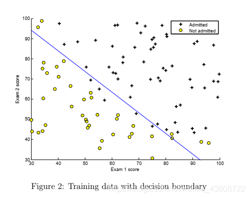
plotDecisionBoundary(theta, X, y);

% Put some labels 
hold on;
% Labels and Legend
xlabel('Exam 1 score')
ylabel('Exam 2 score')

% Specified in plot order
legend('Admitted', 'Not admitted')
hold off;

fprintf('\nProgram paused. Press enter to continue.\n');
pause;

%% ============== Part 4: Predict and Accuracies ==============
%  After learning the parameters, you'll like to use it to predict the outcomes
%  on unseen data. In this part, you will use the logistic regression model
%  to predict the probability that a student with score 45 on exam 1 and 
%  score 85 on exam 2 will be admitted.
%
%  Furthermore, you will compute the training and test set accuracies of 
%  our model.
%
%  Your task is to complete the code in predict.m

%  Predict probability for a student with score 45 on exam 1 
%  and score 85 on exam 2 

prob = sigmoid([1 45 85] * theta);
fprintf(['For a student with scores 45 and 85, we predict an admission ' ...
         'probability of %f\n'], prob);
fprintf('Expected value: 0.775 +/- 0.002\n\n');

% Compute accuracy on our training set
p = predict(theta, X);

fprintf('Train Accuracy: %f\n', mean(double(p == y)) * 100);
fprintf('Expected accuracy (approx): 89.0\n');
fprintf('\n');

2 Regularized logistic regression

在练习的这一部分中，您将实现正则化的逻辑回归来预测来自制造工厂的微芯片是否通过质量保证(QA)。在QA期间，每个微芯片都要经过各种测试，以确保其正常工作。

假设您是工厂的产品经理，您有一些微芯片在两个不同测试中的测试结果。通过这两个测试，您将确定是否应该接受或拒绝微芯片。为了帮助您做出决定，您有一个关于过去微芯片的测试结果的数据集，您可以从该数据集构建逻辑回归模型

2.1 Visualizing the data

与本练习前面的部分类似，plotData.m用于生成如图3所示的图

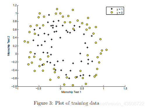
图3显示，我们的数据集不能通过一条直线将其分割为正示例和负示例。因此，直接应用逻辑回归在这个数据集中不会有很好的效果，因为逻辑回归只能找到一个线性的决策边界

2.2 Feature mapping

更好地适应数据的一种方法是从每个数据点创建更多的特性。在提供的函数mapFeature.m，我们将把特征映射到所有x1和x2的多项式项直到六次方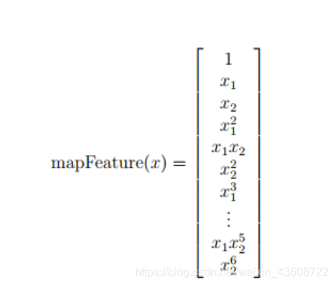

作为映射的结果，我们的两个特征向量(两个QA测试的分数)被转换为一个28维向量。在这个高维特征向量上训练的逻辑回归分类器将会有一个更复杂的决策边界，并且在我们的二维图中会出现非线性。

虽然特征映射允许我们构建一个表达性更强的分类器，但它也更容易发生过拟合。在本练习的下一部分中，您将实现正则逻辑回归来拟合数据，并亲自了解正则化如何帮助解决过拟合问题。

mapFeature.m

function out = mapFeature(X1, X2)
% MAPFEATURE Feature mapping function to polynomial features
%
%   MAPFEATURE(X1, X2) maps the two input features
%   to quadratic features used in the regularization exercise.
%
%   Returns a new feature array with more features, comprising of 
%   X1, X2, X1.^2, X2.^2, X1*X2, X1*X2.^2, etc..
%
%   Inputs X1, X2 must be the same size
%

degree = 6;
out = ones(size(X1(:,1)));
for i = 1:degree
    for j = 0:i
        out(:, end+1) = (X1.^(i-j)).*(X2.^j); %end+1表示向后添加
    end
end

end

2.3 Cost function and gradient

现在，您将实现用于计算正则逻辑回归的成本函数和梯度的代码。在costFunctionReg.m中完成代码。返回代价和梯度。

回想一下logistic回归中的正则化代价函数是
$$J(\theta )=\frac{1}{m}\sum _{i=1}^m[-y^{(i)}log(h_{\theta }(x^i))-(1-y^{(i)})log(1-h_{\theta }(x^i))]+\frac{\lambda }{2m}\sum _{j=1}^n{\theta }_j^2$$
请注意，不应该将参数frof0规范化。在Octave/MATLAB中，索引是从1开始的.因此，您不应该正则化代码中的theta(1)参数(对应于θ0)。代价函数的梯度为向量，其中第j个元素定义如下:
$$\frac{\partial J(\theta )}{\partial {\theta }_j}=\frac{1}{m}\sum _{i=1}^m(h_{\theta }(x^{(i)}-y^{(i)})x_j^{(i)}forj=0$$

$$\frac{\partial J(\theta )}{\partial {\theta }_j}=\frac{1}{m}\sum _{i=1}^m(h_{\theta }(x^{(i)}-y^{(i)})x_j^{(i)}+\frac{\lambda }{m}\sum _{j=1}^n{\theta }_{j}forj⩾1$$

```costFunctionReg.m``

function [J, grad] = costFunctionReg(theta, X, y, lambda)
%COSTFUNCTIONREG Compute cost and gradient for logistic regression with regularization
%   J = COSTFUNCTIONREG(theta, X, y, lambda) computes the cost of using
%   theta as the parameter for regularized logistic regression and the
%   gradient of the cost w.r.t. to the parameters. 

% Initialize some useful values
m = length(y); % number of training examples

% You need to return the following variables correctly 
J = 0;
grad = zeros(size(theta));

% ====================== YOUR CODE HERE ======================
% Instructions: Compute the cost of a particular choice of theta.
%               You should set J to the cost.
%               Compute the partial derivatives and set grad to the partial
%               derivatives of the cost w.r.t. each parameter in theta



theta_1=[0;theta(2:end)];    % 先把theta(1)拿掉，不参与正则化

J=1/m*sum(-y.*log(sigmoid(X*theta))-(1-y).*log(1-sigmoid(X*theta)))+lambda/(2*m)*sum(theta_1.^2);

grad = ( X' * (sigmoid(X*theta) - y ) )/ m + lambda/m * theta_1 ;


% =============================================================

end

2.4 Plotting the decision boundary

为了帮助您可视化这个分类器学习的模型，我们提供了函数plotDecisionBoundary.m，它绘制(非线性)决定边界，分隔正的和负的例子。在plotDecisionBoundary.m，我们在均匀间隔的网格上计算分类器的预测，绘制非线性决策边界，并绘制预测y = 0到y = 1之间的等值线图。

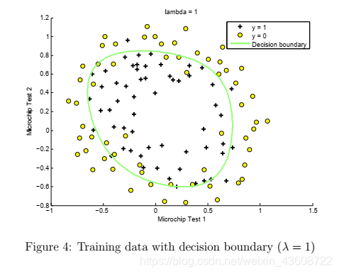
在学习了参数后，下一步在ex_reg.m将绘制一个类似于图4的决策边界。

```ex2_reg.m``

%% Machine Learning Online Class - Exercise 2: Logistic Regression
%
%  Instructions
%  ------------
%
%  This file contains code that helps you get started on the second part
%  of the exercise which covers regularization with logistic regression.
%
%  You will need to complete the following functions in this exericse:
%
%     sigmoid.m
%     costFunction.m
%     predict.m
%     costFunctionReg.m
%
%  For this exercise, you will not need to change any code in this file,
%  or any other files other than those mentioned above.
%

%% Initialization
clear ; close all; clc

%% Load Data
%  The first two columns contains the X values and the third column
%  contains the label (y).

data = load('ex2data2.txt');
X = data(:, [1, 2]); y = data(:, 3);

plotData(X, y);

% Put some labels
hold on;

% Labels and Legend
xlabel('Microchip Test 1')
ylabel('Microchip Test 2')

% Specified in plot order
legend('y = 1', 'y = 0')
hold off;


%% =========== Part 1: Regularized Logistic Regression ============
%  In this part, you are given a dataset with data points that are not
%  linearly separable. However, you would still like to use logistic
%  regression to classify the data points.
%
%  To do so, you introduce more features to use -- in particular, you add
%  polynomial features to our data matrix (similar to polynomial
%  regression).
%

% Add Polynomial Features

% Note that mapFeature also adds a column of ones for us, so the intercept
% term is handled
X = mapFeature(X(:,1), X(:,2));

% Initialize fitting parameters
initial_theta = zeros(size(X, 2), 1);

% Set regularization parameter lambda to 1
lambda = 1;

% Compute and display initial cost and gradient for regularized logistic
% regression
[cost, grad] = costFunctionReg(initial_theta, X, y, lambda);

fprintf('Cost at initial theta (zeros): %f\n', cost);
fprintf('Expected cost (approx): 0.693\n');
fprintf('Gradient at initial theta (zeros) - first five values only:\n');
fprintf(' %f \n', grad(1:5));
fprintf('Expected gradients (approx) - first five values only:\n');
fprintf(' 0.0085\n 0.0188\n 0.0001\n 0.0503\n 0.0115\n');

fprintf('\nProgram paused. Press enter to continue.\n');
pause;

% Compute and display cost and gradient
% with all-ones theta and lambda = 10
test_theta = ones(size(X,2),1);
[cost, grad] = costFunctionReg(test_theta, X, y, 10);

fprintf('\nCost at test theta (with lambda = 10): %f\n', cost);
fprintf('Expected cost (approx): 3.16\n');
fprintf('Gradient at test theta - first five values only:\n');
fprintf(' %f \n', grad(1:5));
fprintf('Expected gradients (approx) - first five values only:\n');
fprintf(' 0.3460\n 0.1614\n 0.1948\n 0.2269\n 0.0922\n');

fprintf('\nProgram paused. Press enter to continue.\n');
pause;

%% ============= Part 2: Regularization and Accuracies =============
%  Optional Exercise:
%  In this part, you will get to try different values of lambda and
%  see how regularization affects the decision coundart
%
%  Try the following values of lambda (0, 1, 10, 100).
%
%  How does the decision boundary change when you vary lambda? How does
%  the training set accuracy vary?
%

% Initialize fitting parameters
initial_theta = zeros(size(X, 2), 1);

% Set regularization parameter lambda to 1 (you should vary this)
lambda = 1;

% Set Options
options = optimset('GradObj', 'on', 'MaxIter', 400);

% Optimize
[theta, J, exit_flag] = ...
	fminunc(@(t)(costFunctionReg(t, X, y, lambda)), initial_theta, options);

% Plot Boundary
plotDecisionBoundary(theta, X, y);
hold on;
title(sprintf('lambda = %g', lambda))

% Labels and Legend
xlabel('Microchip Test 1')
ylabel('Microchip Test 2')

legend('y = 1', 'y = 0', 'Decision boundary')
hold off;

% Compute accuracy on our training set
p = predict(theta, X);

fprintf('Train Accuracy: %f\n', mean(double(p == y)) * 100);
fprintf('Expected accuracy (with lambda = 1): 83.1 (approx)\n');

2.5 Optional (ungraded) exercises

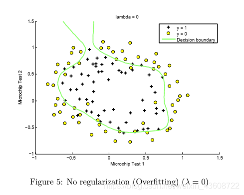
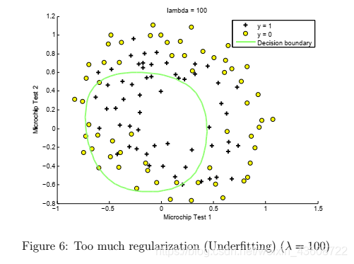
在本部分的练习中，您将为数据集尝试不同的正则化参数，以了解正则化如何防止过拟合。注意决策边界在您变化时的变化。当有一个小的小段时，你会发现分类器几乎得到了每个训练示例的正确值，但却绘制了一个非常复杂的边界，从而过度拟合了数据(图5)。这不是一个好的边界决策:例如，它预测了x = (-0.25,1:5)被接受(y = 1)，这似乎是一个不正确的决策给定的训练集。有一个更大的数据集，您应该看到一个图，显示了一个更简单的决策边界，仍然可以很好地分离积极和消极。但是，如果将该值设置得过高，则无法很好地拟合，决策边界也不会很好地跟随数据，从而导致拟合数据不足(图6)。