【Andrew Gelman Data Analysis Using Regression and Multilevel/Hierarchical Models】2.8 exercises 解答

自己写的答案，希望各位朋友们多加批评指正

第一题

1. A test is graded from 0 to 50, with an average score of 35 and a standard deviation of 10. For comparison to other tests, it would be convenient to rescale to a mean of 100 and standard deviation of 15.
   (a) How can the scores be linearly transformed to have this new mean and standard deviation?
   (b) There is another linear transformation that also rescales the scores to have mean 100 and standard deviation 15. What is it, and why would you not want to use it for this purpose?

#生成均值为35方差为10的正态分布序列
V1 <- rnorm(100,mean=35,sd=10)
#计算z-score(这里可能均值不完全为0，但是是一个很小的数。方差也只是趋近于1)
V1_z <- (V1-mean(V1))/sd(V1)
#利用z-score对数据进行rescale
#成为均值100，标准差15的新的数组
V2 <- V1_z*15+100

第二题

2. The following are the proportions of girl births in Vienna for each month in 1908 and 1909 (out of an average of 3900 births per month):
   .4777 .4875 .4859 .4754 .4874 .4864 .4813 .4787 .4895 .4797 .4876 .4859
   .4857 .4907 .5010 .4903 .4860 .4911 .4871 .4725 .4822 .4870 .4823 .4973
   The data are in the folder girls. von Mises (1957) used these proportions to claim that the sex ratios were less variable than would be expected by chance.
   (a) Compute the standard deviation of these proportions and compare to the standard deviation that would be expected if the sexes of babies were independently decided with a constant probability over the 24-month period.
   (b) The actual and theoretical standard deviations from (a) differ, of course. Is this difference statistically significant? (Hint: under the randomness model, the actual variance should have a distribution with expected value equal to the theoretical variance, and proportional to a χ2 with 23 degrees of freedom.)

$T是这道题要求的实际标准差$
$T^{theory}是这道题要求的理论值标准差$

• 第一步：计算T与T的理论值
  $T=s{d}_{t=1}^{24}{p}_t=0.006416639$
  $T^{theory}=\sqrt{\pi (1-\pi )\times \frac{1}{n}}$ $,n=3000$
  $在这里\pi 是总体中的均值，所以我们用样本的均值p代替$
  $p=av{g}_{t=1}^{24}{p}_t=0.485575$
  $T^{theory}=0.009124909$
• 第二步：计算卡方值
  ${\chi }^2=\frac{{\sum }_{t=1}^6(T-T^{theory}{)}^2}{T^{theory}}=0.0008038137$
  $卡方值的自由度为t-1=23，这个值太小了完全不显著$
  $因此无法拒绝H_0，婴儿性别与出生的月份相互独立$

setwd("/Users/wangningzhi/Desktop")
data1 <- read.csv("./2.8exercise-2data.csv",header = F)
#给变量赋值
girls <- data1$V1
n <- 3000

#题目：计算出生月份与性别是否独立
#1、计算实际值标准差
T <- sqrt(var(girls))
#2、计算样本的均值
p_i <- sum(girls)/length(girls)
#3、计算理论值标准差
T_theory <- sqrt(p_i*(1-p_i)/n)
#4、计算卡方值
chi_square <- sum((T-T_theory)^2)/T_theory

第三题

3. Demonstration of the Central Limit Theorem: let x = x1 + ··· + x20, the sum of 20 independent Uniform(0,1) random variables. In R, create 1000 simulations of x and plot their histogram. On the histogram, overlay a graph of the normal density function. Comment on any differences between the histogram and the curve.

#设置每个组的个体数
n.x <- 20
#生成
#设置组的均值
p.hat.x <- 0
#设置组的标准误，即均值的标准差
se.x <- sqrt(1/n.x)
#设置模拟的次数（抽样次数）
n.sim <- 1000
#先生成n.sim个均值为0，方差为均值标准误的正态分布随机数
p.x <- rnorm(n.sim,mean=0,sd=se.x)
#将这20个随机数求和
p.x.sum <- sum(p.x)
#绘制散点图
hist(p.x, breaks=100)
#叠加normal的概率密度曲线
par(new=TRUE)
lines(plot(dnorm,-1,1))

叠加后发现，均值组成的分布较标准正态分布更为收敛，即更加集中趋向于0。

第四题

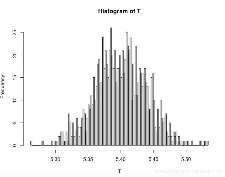
4. Distribution of averages and differences: the heights of men in the United States are approximately normally distributed with mean 69.1 inches and standard deviation 2.9 inches. The heights of women are approximately normally distributed with mean 63.7 inches and standard deviation 2.7 inches. Let x be the average height of 100 randomly sampled men, and y be the average height of 100 randomly sampled women. In R, create 1000 simulations of x − y and plot their histogram. Using the simulations, compute the mean and standard deviation of the distribution of x − y and compare to their exact values.

#设置每组样本个数
n.men <- 100
n.women <- 100
#设置组的标准误
se.men <- 2.9/n.men
se.women <- 2.7/n.women
#设置组的均值
hat.men <- 69.1
hat.women <- 63.7
#拟合1000个组
n.sim <- 1000
p.men <- rnorm(n.sim,mean=hat.men,sd=se.men)
p.women <- rnorm(n.sim,mean=hat.women,sd=se.women)
#计算p.men-p.women统计量T
T <- p.men-p.women
#绘制直方图
hist(T,breaks=100)
#计算均值和标准差
p.men_mean <- mean(p.men)
p.men_sd <- sd(p.men)
p.women_mean <- mean(p.women)
p.women_sd <- sd(p.women)
#计算其与真值的差异
m.mean.diff <- p.men_mean - hat.men
m.sd.diff <- p.men_sd - se.men
wm.mean.diff <- p.women_mean - hat.women
wm.sd.diff <- p.women_sd - se.women
#打印结果
x <- c(m.mean.diff,m.sd.diff,wm.mean.diff,wm.sd.diff)
print(x)

第五题

5. Correlated random variables: suppose that the heights of husbands and wives have a correlation of 0.3. Let x and y be the heights of a married couple chosen at random. What are the mean and standard deviation of the average height, (x + y)/2?

这道题没给均值是不可能算出确切值的，因为D(X+Y)=D(X)+D(Y)+2Cov(X,Y)，只能带入Cov(X,Y)=0.3。
但是二者之和的期望和方差可以用回归公式表示。
在OLS回归中，

$\hat{y}=\hat{\alpha }+\hat{\beta }\hat{x}+\hat{\mu }$

$这里\hat{\alpha }是回归直线的斜率，\hat{\beta }是\hat{x}和\hat{y}的相关系数$
$\hat{\mu }是误差项，我们设误差项的标准误为\hat{\sigma }$

$\frac{\hat{x}+\hat{y}}{2}=\frac{\hat{\alpha }+\hat{\beta }\hat{x}+\hat{\mu }+\hat{x}}{2}=\frac{\hat{\alpha }}{2}+(\frac{\hat{\beta }+1}{2})\hat{x}+\frac{\hat{\mu }}{2}$

$题目给出\hat{\beta }=0.3，还需要知道\hat{\alpha }和\hat{x}才能算出\frac{\hat{x}+\hat{y}}{2}的期望$