【动手学习pytorch笔记】1.线性回归

Liner回归的从零实现

%matplotlib inline
import random
import torch
from d2l import torch as d2l

生成一个人造数据集

def synthetic_data(w, b, num_examples):  #@save
    """生成y=Xw+b+噪声"""
    X = torch.normal(0, 1, (num_examples, len(w)))
    y = torch.matmul(X, w) + b
    y += torch.normal(0, 0.01, y.shape)
    return X, y.reshape((-1, 1))

true_w = torch.tensor([2, -3.4])
true_b = 4.2
features, labels = synthetic_data(true_w, true_b, 1000)

X：二维矩阵（样本数 * 特征长度）1000 * 2

y：向量 1000 * 1

+b是广播机制

真实值： true_w = torch.tensor([2, -3.4])
true_b = 4.2

y += torch.normal(0, 0.01, y.shape)：随机噪音

print('features:', features[0],'\nlabel:', labels[0])

features: tensor([-0.1284, -0.6457]) 
label: tensor([6.1244])

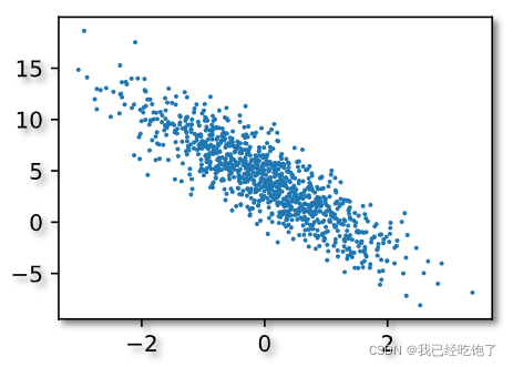
d2l.set_figsize()
d2l.plt.scatter(features[:, 1].detach().numpy(), labels.detach().numpy(), 1);

读取数据集

def data_iter(batch_size, features, labels):
    num_examples = len(features)
    indices = list(range(num_examples))
    # 这些样本是随机读取的，没有特定的顺序
    random.shuffle(indices)
    for i in range(0, num_examples, batch_size):
        batch_indices = torch.tensor(
            indices[i: min(i + batch_size, num_examples)])
        yield features[batch_indices], labels[batch_indices]

data_iter用来拿batch_size个样本

​ num_examples = 1000

​ indices 包含所有样本下标的列表，被打乱

​ ==for i in range(0, num_examples, batch_size)：==每隔batch_size个拿一个下标i

​ 获得i之后，往后取batch_size个，yield(return)出去

​ ==min(i + batch_size, num_examples)：==最后一组可能不够batch_size个，那就全拿了

batch_size = 10

for X, y in data_iter(batch_size, features, labels):
    print(X, '\n', y)
    break

因为这里break了，所以只yield了一组

tensor([[ 1.2599, -0.9327],
        [ 1.1232,  0.2566],
        [-0.3754,  0.7046],
        [-0.6855, -1.2303],
        [ 1.5169, -0.0099],
        [ 0.0754,  1.1267],
        [ 0.1643, -0.0296],
        [-0.7567,  0.5444],
        [ 0.2624,  0.4333],
        [-1.9114,  0.3921]]) 
 tensor([[ 9.8939],
        [ 5.5723],
        [ 1.0727],
        [ 6.9968],
        [ 7.2692],
        [ 0.5038],
        [ 4.6170],
        [ 0.8265],
        [ 3.2630],
        [-0.9715]])

初始化模型参数

w = torch.normal(0, 0.01, size=(2,1), requires_grad=True)
b = torch.zeros(1, requires_grad=True)

定义模型

def linreg(X, w, b):  
    """线性回归模型"""
    return torch.matmul(X, w) + b

定义损失函数

def squared_loss(y_hat, y):  
    """均方损失"""
    return (y_hat - y.reshape(y_hat.shape)) ** 2 / 2

这里损失函数没有求均值，所以下面梯度下降的时候求了均值，一样的。

定义优化算法

def sgd(params, lr, batch_size):  
    """小批量随机梯度下降"""
    with torch.no_grad():
        for param in params:
            param -= lr * param.grad / batch_size
            param.grad.zero_()

训练

lr = 0.03
num_epochs = 3
net = linreg
loss = squared_loss

for epoch in range(num_epochs):
    for X, y in data_iter(batch_size, features, labels):
        l = loss(net(X, w, b), y)  # X和y的小批量损失
        # 因为l形状是(batch_size,1)，而不是一个标量。l中的所有元素被加到一起，
        # 并以此计算关于[w,b]的梯度
        l.sum().backward()
        sgd([w, b], lr, batch_size)  # 使用参数的梯度更新参数
    with torch.no_grad():
        train_l = loss(net(features, w, b), labels)
        print(f'epoch {epoch + 1}, loss {float(train_l.mean()):f}')

epoch 1, loss 0.034527
epoch 2, loss 0.000121
epoch 3, loss 0.000046

比较真实的w,b和模型学习到的差距

print(f'w的估计误差: {true_w - w.reshape(true_w.shape)}')
print(f'b的估计误差: {true_b - b}')

w的估计误差: tensor([ 0.0003, -0.0007], grad_fn=<SubBackward0>)
b的估计误差: tensor([0.0011], grad_fn=<RsubBackward1>)

Liner回归简易实现

import numpy as np
import torch
from torch.utils import data
from d2l import torch as d2l
from torch import nn

true_w = torch.tensor([2,-3.4])
true_b = 4.2
features,labels = d2l.synthetic_data(true_w,true_b,1000)

def load_array(data_arrays, batch_size, is_train = True):
    dataset = data.TensorDataset(*data_arrays)
    return data.DataLoader(dataset, batch_size, shuffle = is_train)

batch_size = 10
data_iter = load_array((features,labels), batch_size)

next(iter(data_iter))

输出

[tensor([[ 0.3478, -0.1429],
         [-0.1305,  0.9412],
         [-0.9198, -0.4407],
         [-0.7321, -0.1986],
         [-1.3152, -0.3509],
         [-1.0748,  0.5044],
         [ 0.8715, -0.2265],
         [-1.0149,  0.7534],
         [-0.2333, -0.2114],
         [-1.7907,  1.2627]]),
 tensor([[ 5.3866],
         [ 0.7402],
         [ 3.8383],
         [ 3.4077],
         [ 2.7556],
         [ 0.3289],
         [ 6.7145],
         [-0.3806],
         [ 4.4456],
         [-3.6826]])]

net = nn.Sequential(nn.Linear(2,1))

net[0].weight.data.normal_(0,0.01)
net[0].bias.data.fill_(0)

==nn.Linear(2,1)：==X的维度2，y的维度1

loss = nn.MSELoss()

trainer = torch.optim.SGD(net.parameters(),lr = 0.03)

num_epochs = 3
for epoch in range(num_epochs):
    for X,y in data_iter:
        l = loss(net(X),y)
        trainer.zero_grad()
        l.backward()
        trainer.step()
    l = loss(net(features),labels)
    print(f'epoch{epoch + 1},loss{l:f}')

epoch1,loss0.000327
epoch2,loss0.000103
epoch3,loss0.000103