MATLAB绘图
4.1二维曲线
matlab常用绘图函数
(1)plot函数的基本用法
plot(x,y)
其中,x和y分别用于存储x坐标和y坐标数据。
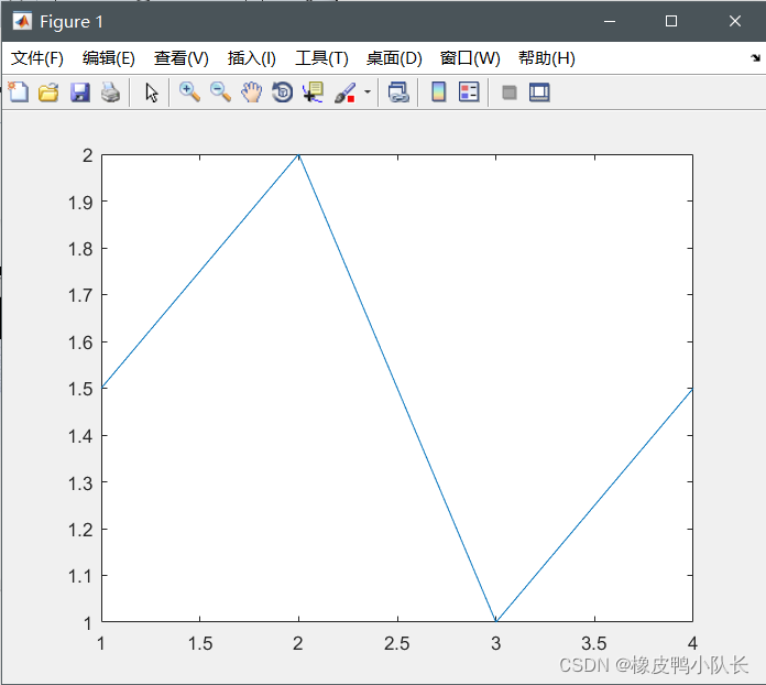
例:绘制一条折线。>> x = [2.5,3.5,4,5]; >> y = [1.5,2.0,1,1.5]; >> plot(x,y)

(2)最简单的plot函数调用格式
plot(x)
>> x = [1.5,2,1,1.5];
>> plot(x)
当plot函数的参数x是复数向量时,则分别以该向量元素实部和虚部为横、纵坐标绘制出一条曲线。
>> x = [1.5,2,1,1.5];
>> plot(x)
>> x = [2.5,3.5,4,5];
>> y = [1.5,2,1,1.5];
>> cx = x+y*i;
>> plot(cx)

(3)polot(x,y)函数参数的变化形式
当x是向量,y是矩阵时
如果矩阵y的列数等于x的长度,则以向量x为横坐标,以y的每个行向量为纵坐标绘制坐标曲线,曲线的条数等于y的行数。
如果矩阵y的行数等于x的长度,则以向量x为横坐标,以y的每个列向量为纵坐标绘制坐标曲线,曲线的条数等于y的列数。
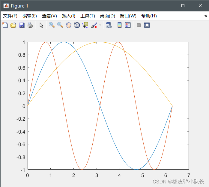
例:绘制sinx、sin(2x)、sin(x/2)的函数曲线。>> x = linspace(0,2*pi,100); >> y = [sin(x);sin(2*x);sin(0.5*x)]; >> plot(x,y)
当x、y时同型矩阵时,以x、y对应列元素为横、纵坐标分别绘制曲线,曲线条数等于矩阵的列数。
(3)plot(x,y)函数参数的变化形式
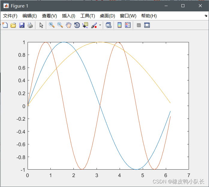
>> t = 0:0.1:2*pi;
>> t1 = t';
>> x = [t1,t1,t1];
>> y = [sin(t1),sin(2*t1),sin(0.5*t1)];
>> plot(x,y)
(4)含多个输入参数的plot函数
plot(x1,y1,x2,y3,…,xn,yn)
其中,每一向量对构成一组数据点的横、纵坐标,绘制一条曲线。
>> t1=linspace(0,2*pi,10);
>> t2=linspace(0,2*pi,20);
>> t3=linspace(0,2*pi,100);
>> plot(t1,sin(t1),t2,sin(t2)+1,t3,sin(t3)+2)
(5)含选项的plot函数
plot(x,y,选项)
| 线型 | 颜色 | 数据点标记 |
|---|---|---|
| “-”:实线 | “r”:红色 | "*"星号 |
| “:”:虚线 | “g”:绿色 | “o”:圆圈 |
| “-.”:点画线 | “b”:蓝色 | “s”:方块 |
| “–”:双画线 | “k”:黑色 | “p”:五角星 |
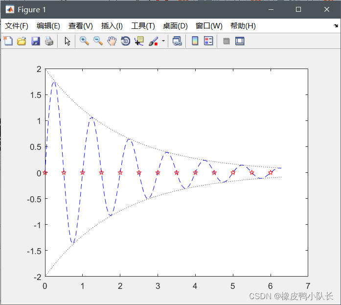
*例:用不同线型和颜色在同一坐标内绘制曲线y = 2 e − 0.5 x sin 2 π x y=2e^{-0.5x}\sin{2\pi x}y=2e−0.5xsin2πx*及其包络线。
x=(0:pi/50:2*pi);
y1=2*exp(-0.5*x).*[1;-1];
y2=2*exp(-0.5*x).*sin(2*pi*x);
x1=0:0.5:6;
y3=2*exp(-0.5*x1).*sin(2*pi*x1);
plot(x,y1,'k:',x,y2,'b--',x1,y3,'rp')
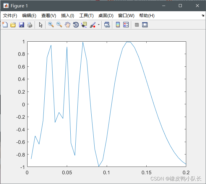
例:绘制函数sin 1 x \sin{\frac{1}{x}}sinx1的图形。
>> x=0:0.005:0.2;
>> y=sin(1./x);
>> plot(x,y)
- fplot函数(根据函数特性,自适应产生采样间隔)
(1)基本用法
fplot(f,lims,选项)
f代表一个函数,通常采用函数句柄的形式。lims为x轴的取值范围,用二元向量[xmin,xmax]描述,默认值为[-5,5]。选项定义与plot函数相同。
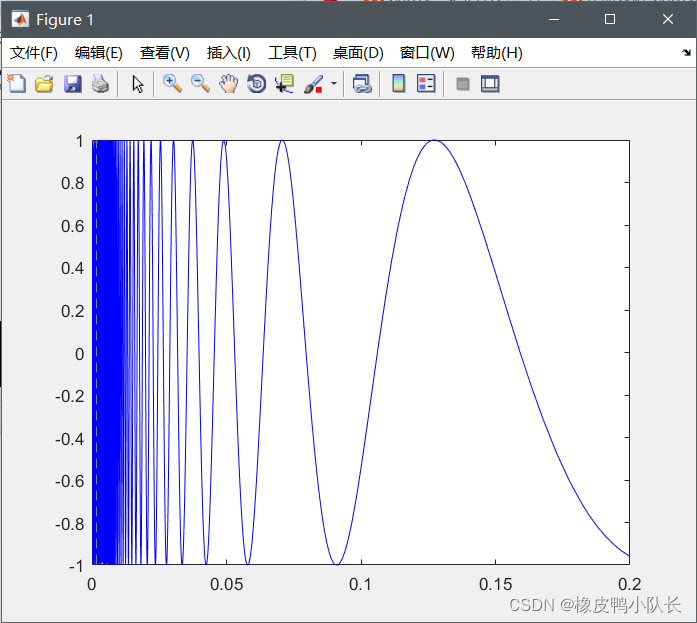
*例:采用fplot函数绘制函数sin 1 x \sin{\frac{1}{x}}sinx1的图形。
>> fplot(@(x)sin(1./x),[0,0.2],'b')
(2)双输入函数参数的用法
fplot(funx,funy,tlims,选项)
funx、funy代表函数,通常采用函数句柄的形式。
tlims为参数函数funx和funy的自变量的取值范围,用二元向量[tmin,tmax]描述。
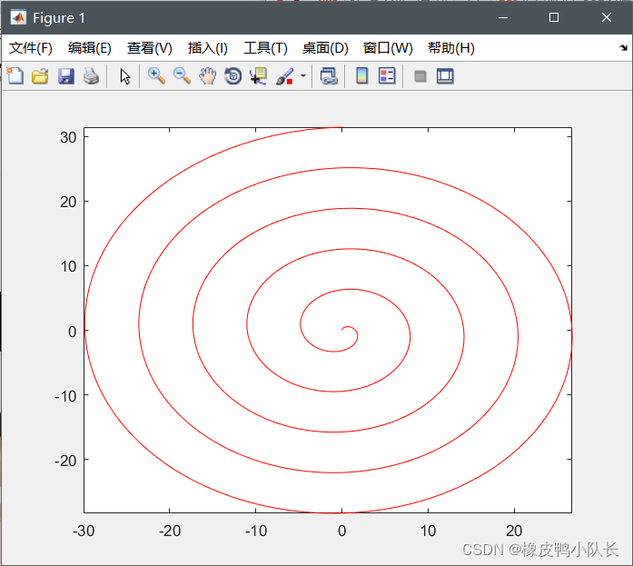
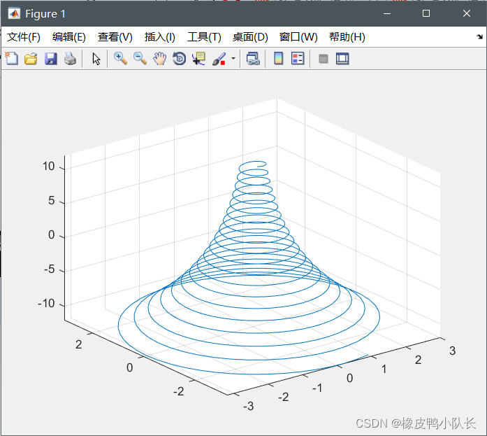
*例:已知螺旋线的参数方程,绘制曲线。
{ x = t ⋅ s i n t y = t ⋅ c o s t \begin{cases} x=t \cdot sint \\ y=t \cdot cost \end{cases}{x=t⋅sinty=t⋅cost
>> fplot(@(t)t.*sin(t),@(t)t.*cos(t),[0,10*pi],'r')
4.2绘制图形的辅助操作
给图形添加标注
title(图形标题)
xlabel(x轴说明)
ylabel(y轴说明)
text(x,y,图形说明)
legend(图例1,图例2,…)
- title函数
①title函数的基本用法
title(图形标题)
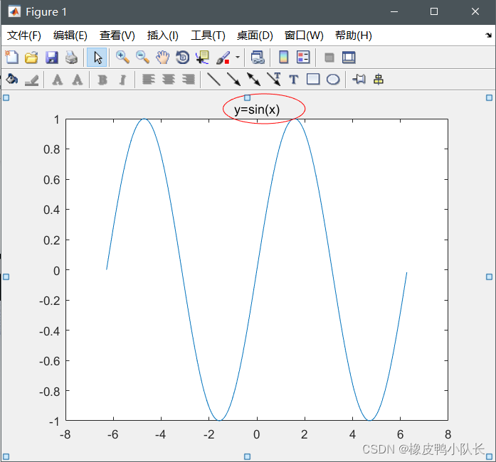
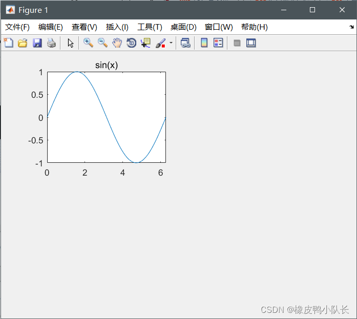
例:绘制[ − 2 π , 2 π ] [-2\pi,2\pi][−2π,2π]区间的正弦曲线并给图形添加标题。
>> x=-2*pi:0.05:2*pi;
>> y=sin(x);
>> plot(x,y)
>> title('y=sin(x)')
②在图形标题中使用Latex格式控制符
>>title(‘y=cos{\omega}t’)
>>title('y=e^{axt}')
>>title('X_{1}{\geq}X_{2}')
>>title('{\bf y=cos{\omega}t+{\beta}}')
③含属性设置的title函数
title(图形标题,属性名,属性值)
Color属性:
>>title('y=cos{\omega}t','Color','r')
FontSize属性:
>>title('y=cos{\omega}t','FontSize',24 )
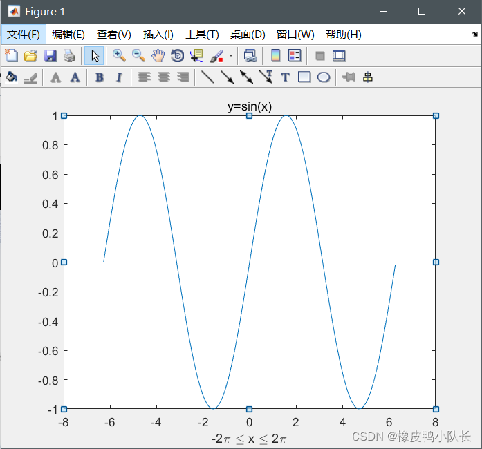
xlabel和ylabel函数
>> x=-2*pi:0.05:2*pi;
>> y=sin(x);
>> plot(x,y)
>> title('y=sin(x)')
>> xlabel('-2\pi \leq x \leq 2\pi')
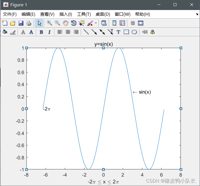
text函数和gtex函数
text(x,y,说明)
gtext(说明)>> text(-2*pi,0,'-2{\pi}') >> text(3,0.28,'\leftarrow sin(x)')
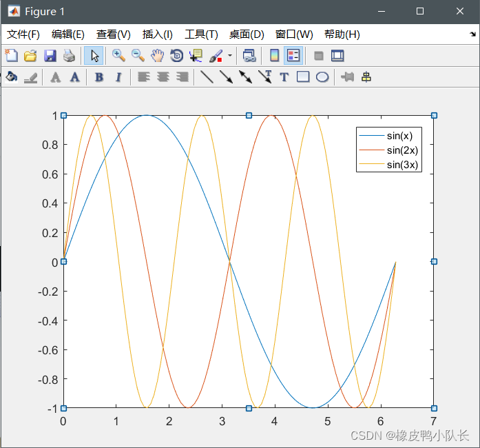
- legend函数zheng
例:绘制不同频率的正弦曲线并用图例标注曲线。
>> x = linspace(0,2*pi,100);
>> plot(x,[sin(x);sin(2*x);sin(3*x)])
>> legend('sin(x)','sin(2x)','sin(3x)')
坐标控制
axis函数
axis([xmin,xmax,ymin,ymax,zmin,zmax])
axis equal:纵、横坐标轴采用等长刻度
axis square:产生正方形坐标系(默认为矩形)
axis auto:使用默认设置
axis off:取消坐标轴
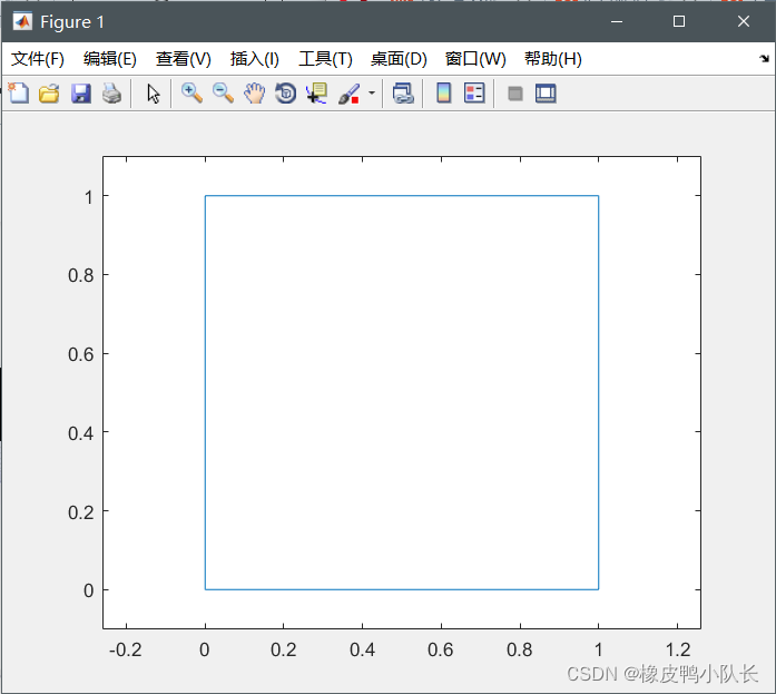
axis on:显示坐标轴>> x=[0,1,1,0,0]; >> y=[0,0,1,1,0]; >> plot(x,y)
>> axis([-0.1,1.1,-0.1,1.1])
>> axis equal;
- 给坐标系加网格和边框
加网格
grid on
grid off
grid
加边框
box on
box off
box
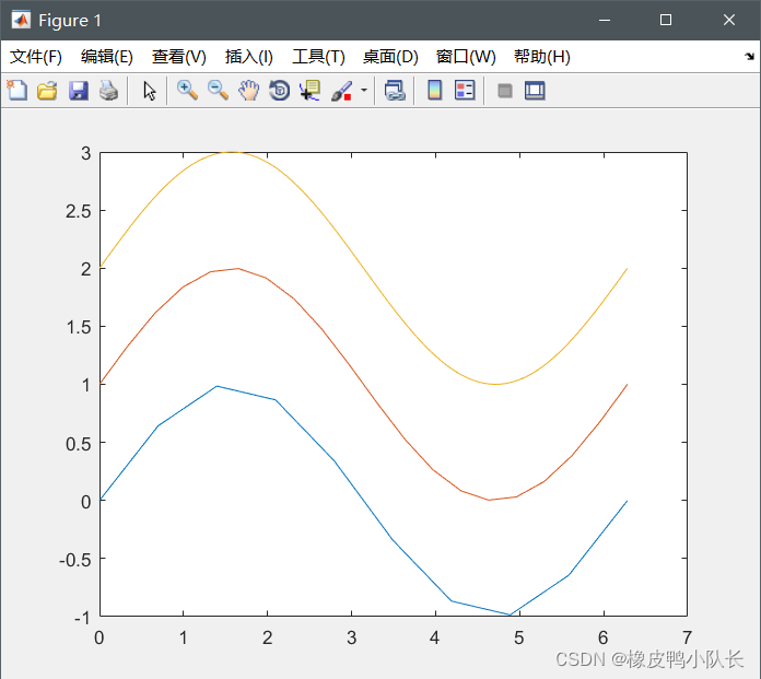
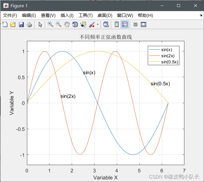
例:绘制sin x \sin xsinx、sin 2 x \sin{2x}sin2x、sin ( x / 2 ) \sin{(x/2)}sin(x/2)的函数曲线并添加图形标注。
>> x=linspace(0,2*pi,100);
>> y=[sin(x);sin(2*x);sin(0.5*x)];
>> plot(x,y)
>> axis([0,7,-1.2,1.2])
>> title('不同频率正弦函数曲线');
>> xlabel('Variable X');ylabel('Variable Y');
>> text(2.5,sin(2.5),'sin(x)');
>> text(1.5,sin(2*1.5),'sin(2x)');
>> text(5.5,sin(0.5*5.5),'sin(0.5x)');
>> legend('sin(x)','sin(2x)','sin(0.5x)');
>> grid on
图形保持
在已存在的图形上添加新图形
hold on
hold off
hold
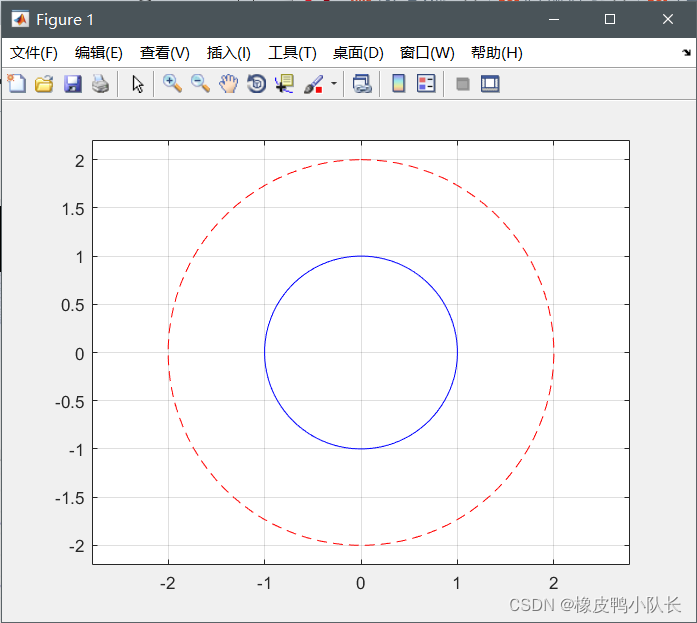
例:用图形保持功能绘制两个同心圆。
>> t=linspace(0,2*pi,100);
>> x=sin(t);y=cos(t);
>> plot(x,y,'b');
>> hold on
>> plot(2*x,2*y,'r--')
>> grid on
>> axis([-2.2,2.2,-2.2,2.2])
>> axis equal
图形窗口的分割
子图:同一图形窗口中不同坐标系下的图形。
subplot函数:
subplot(m,n,p)
m和n将制定图形窗口分成m×n个绘图区,p制定当前活动区。
>> subplot(2,2,1);
>> x=linspace(0,2*pi,60);
>> y=sin(x);
>> plot(x,y)
>> title('sin(x)');
>>> axis([0,2*pi,-1,1]);
>> x=linspace(0,2*pi,60);
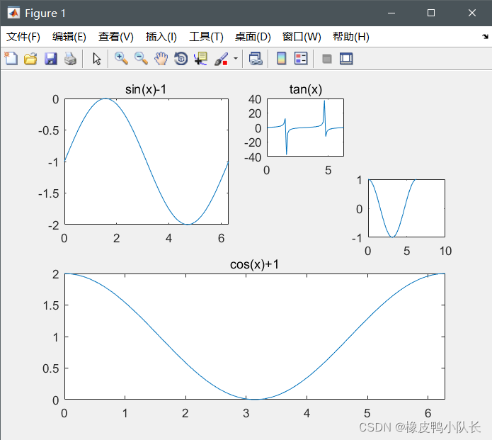
>> subplot(2,2,1)
>> plot(x,sin(x)-1);
>> title('sin(x)-1');axis([0,2*pi,-2,0])
>> subplot(2,1,2)
>> plot(x,cos(x)+1)
>> title('cos(x)+1');axis([0,2*pi,0,2])
>> subplot(4,4,3)
>> plot(x,tan(x));
>> title('tan(x)');axis([0,2*pi,-40,40])
>> subplot(4,4,8)
>> plot(x,cos(x));
>> title('cos(x)');axis([0,2*pi,-35,35])
4.3其他形式的二维图形
其他坐标系下的二维曲线图
- 对数坐标图
semilogx(x1,y1,选项1,x2,y2,选项2,…)
semilogy(x1,y1,选项1,x2,y2,选项2,…)
loglog(x1,y1,选项1,x2,y2,选项2,…)
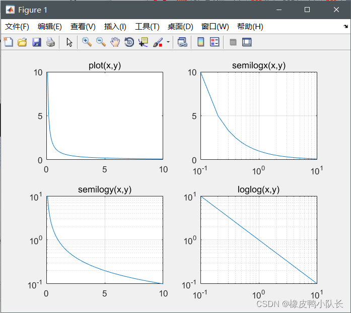
例:绘制1 x \frac{1}{x}x1的直角线性坐标图和三种对数坐标图。
>> x=0:0.1:10;
>> y=1./x;
>> subplot(2,2,1);
>> plot(x,y)
>> title('plot(x,y)');subplot(2,2,2);
>> semilogx(x,y)
>> title('semilogx(x,y)');grid on
>> subplot(2,2,3);
>> semilogy(x,y)
>> title('semilogy(x,y)');grid on
>> subplot(2,2,4);
>> loglog(x,y)
>> title('loglog(x,y)');grid on
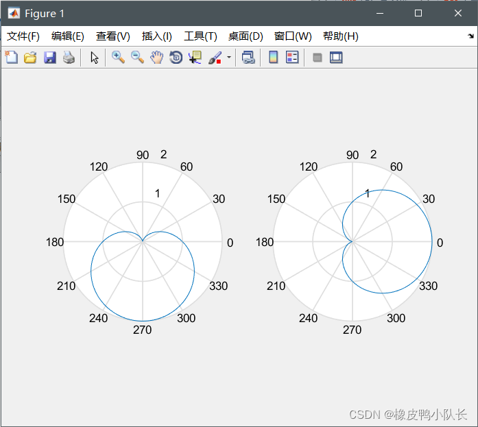
例:按极坐标方程ρ = 1 − sin θ \rho=1-\sin\thetaρ=1−sinθ绘制心形曲线。
>> t=0:pi/100:2*pi;
>> r=1-sin(t);
>> subplot(1,2,1)
>> polar(t,r)
>> subplot(1,2,2)
>> t1=t-pi/2;
>> r1=1-sin(t1);
>> polar(t,r1)
统计图
条形类图
条形图
bar函数
barh函数bar(y,style)
参数y是数据,选项style用于制定分组排列模式。
style:
“grouped”:簇状分组
“stacked”:堆积分组
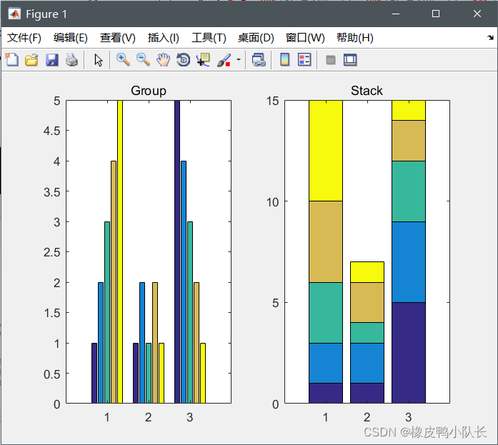
例:绘制分组条形图。
>> y=[1,2,3,4,5;1,2,1,2,1;5,4,3,2,1];
>> subplot(1,2,1)
>> bar(y)
>> title('Group')
>> subplot(1,2,2)
>> bar(y,'stacked')
>> title('Stack')
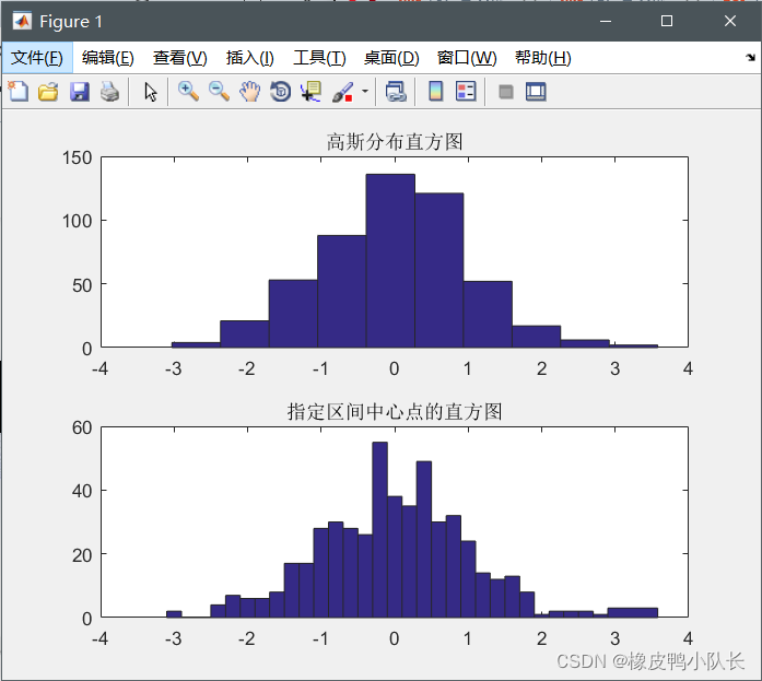
直方图
hist函数
hist(y)
hist(y,x)
其中,参数y是要统计的数据,x用于指定区间的划分方式。
例:绘制服从高斯分布的直方图。>> y=randn(500,1); >> subplot(2,1,1); >> hist(y); >> title('高斯分布直方图'); >> subplot(2,1,2); >> x=-3:0.2:3; >> hist(y,x); >> title('指定区间中心点的直方图')
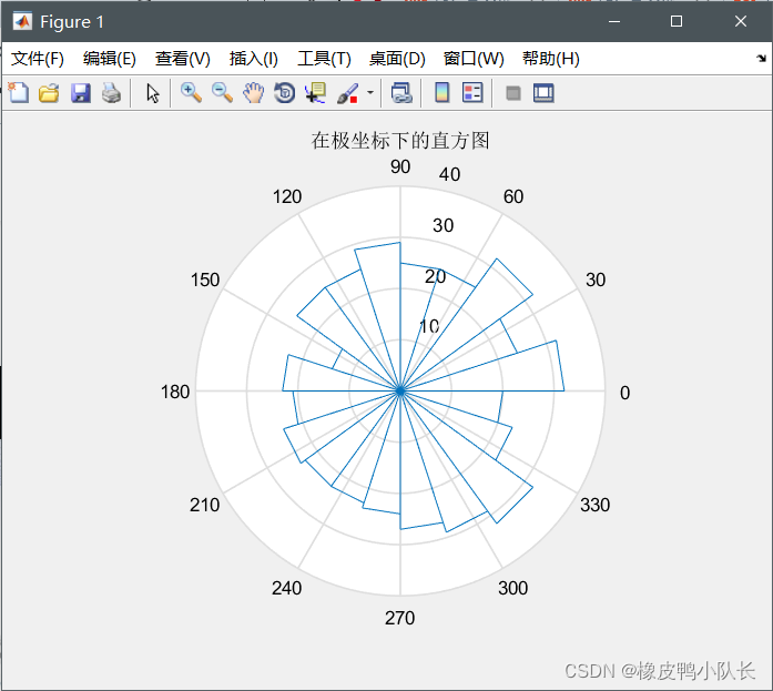
rose函数
rose(theta,x)
其中,参数theta用于确定每一区间与原点的角度,选项x用于指定区间的划分方式。
例:绘制高斯分布数据在极坐标下的直方图。
>> y=randn(500,1);
>> theta=y*pi;
>> rose(theta)
>> title('在极坐标下的直方图')
面积类图形
扇形图
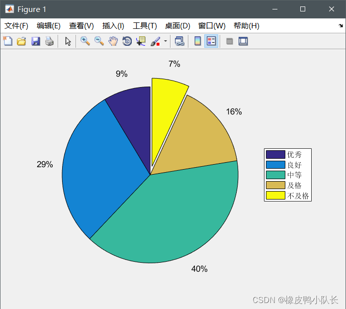
pie函数
pie(x,explode)
其中,参数x存储待统计数据,选项explode控制图块的显示模式。
例:某次考试优秀、良好、中等、及格、不及格的人数分别为:5、17、23、9、4,用扇形统计图作成绩统计分析。>> score=[5,17,23,9,4]; >> ex=[0,0,0,0,1]; >> pie(score,ex) >> legend('优秀','良好','中等','及格','不及格','location','eastoutside')
2. 面积图
area函数
与plot函数用法相同,只是填充了颜色。
散点类图形
scatter函数:散点图
scatter(x,y,选项,‘filled’)
参数x、y用于定位数据点,选项用于指定线型、颜色、数据点标记。
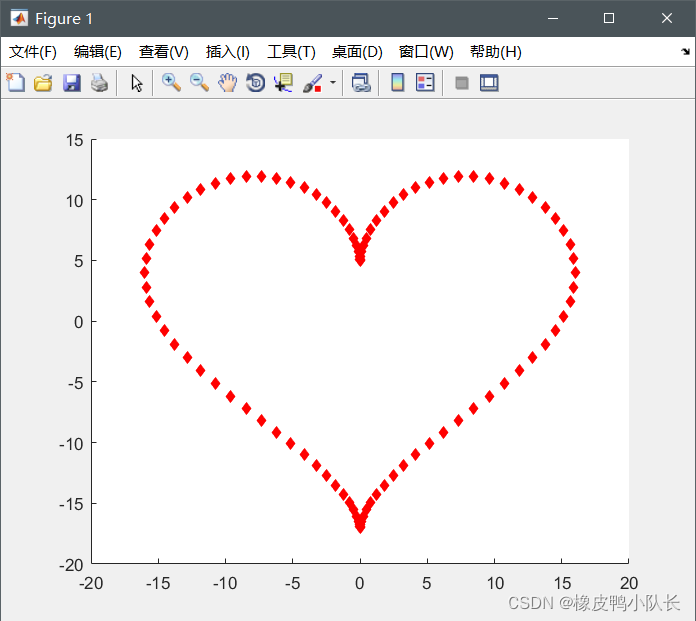
例:以散点图形式绘制桃心曲线,曲线参数方程如下:
{ x = 16 s i n 3 t y = 13 c o s t − 5 c o s ( 2 t ) − 2 c o s ( 3 t ) − c o s ( 4 t ) \begin{cases} x = 16sin^3t\\ y = 13cost-5cos(2t)-2cos(3t)-cos(4t) \end{cases}{x=16sin3ty=13cost−5cos(2t)−2cos(3t)−cos(4t)
>> t=0:pi/50:2*pi;
>> x=16*sin(t).^3;
>> y = 13*cos(t) - 5*cos(2*t) - 2*cos(3*t) - cos(4*t);
>> scatter(x,y,'rd','filled')
stairs函数:阶梯图
stem函数:杆图
矢量图形
compass函数:罗盘图
feather函数:羽毛图
quiver函数:箭头图
quiver(x,y,u,v)
其中,(x,y)指定矢量起点,(u,v)指定矢量终点。
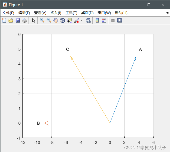
例:已知向量A、B,求A+B,并用矢量图表示。
>> A=[4,5];B=[-10,0];C=A+B;
>> hold on;
>> quiver(0,0,A(1),A(2));
>> quiver(0,0,B(1),B(2));
>> quiver(0,0,C(1),C(2));
>> text(A(1),A(2),'A');
>> text(B(1),B(2),'B');
>> text(C(1),C(2),'C');
>> axis([-12,6,-1,6])
>> grid on
4.4三维曲线
plot3函数
plot3函数基本用法
plot3(x,y,z)
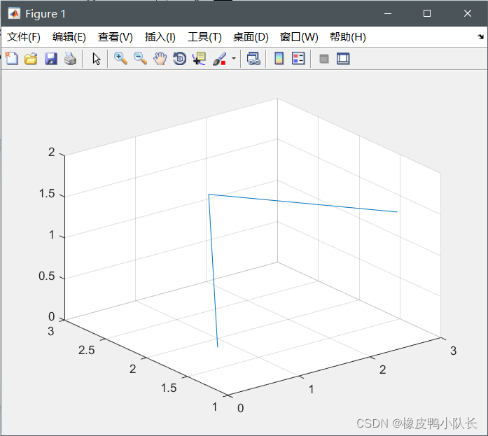
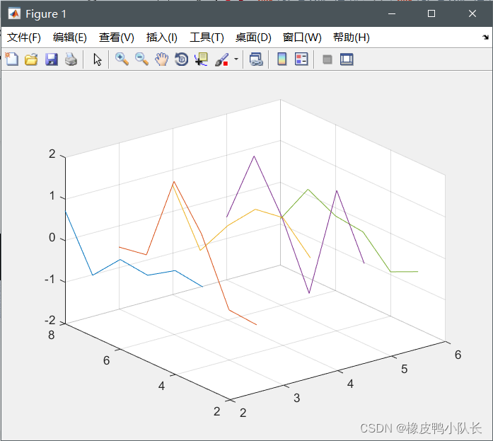
例:绘制一条空间折线。
>> x=[0.2,1.8,2.5];
>> y=[1.3,2.8,1.1];
>> z=[0.4,1.2,1.6];
>> plot3(x,y,z)
>> grid on
>> axis([0,3,1,3,0,2]);
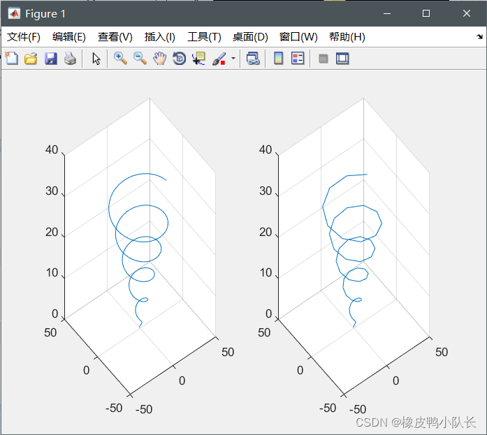
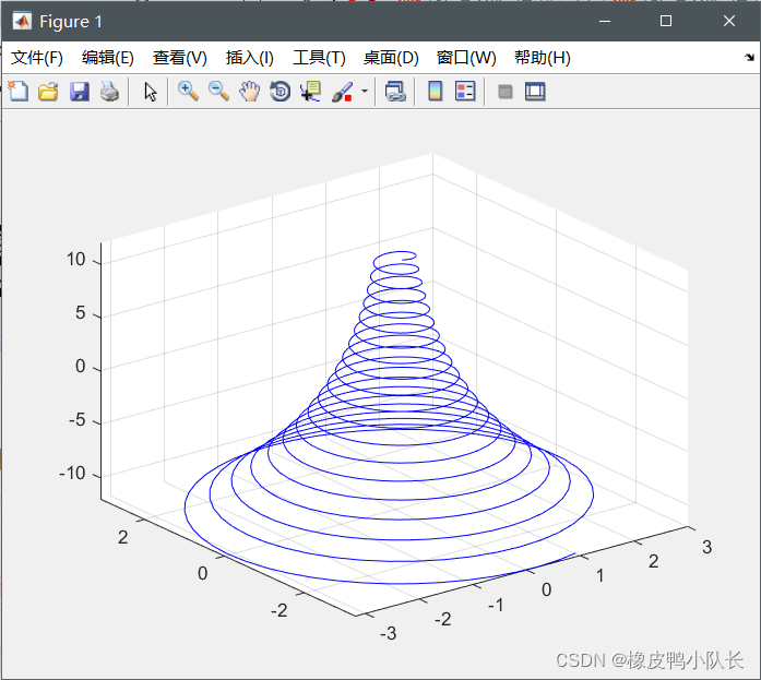
例:绘制螺旋线{ x = s i n t + t ⋅ c o s t y = c o s t − t ⋅ s i n t ( 0 ≤ t ≤ 10 π ) z = t \begin{cases}x=sint+t\cdot cost\\y=cost-t\cdot sint (0\leq t\leq 10\pi)\\z=t\end{cases}⎩⎪⎨⎪⎧x=sint+t⋅costy=cost−t⋅sint(0≤t≤10π)z=t。
>> t=linspace(0,10*pi,200);
>> x=sin(t)+t.*cos(t);
>>y=cos(t)-t.*sin(t);
>>z=t;
>> subplot(1,2,1)
>> plot3(x,y,z)
>> grid on
>> subplot(1,2,2)
>> plot3(x(1:4:200),y(1:4:200),z(1:4:200))
>> grid on
fplot3函数
fplot3(funx,funy,funz,tlims)
例:绘制墨西哥帽顶曲线,曲线参数方程为:{ x = e − t / 10 s i n ( 5 t ) y = = e − t / 10 c o s ( 5 t ) t ∈ [ − 12 , 12 ] z = t \begin{cases}x=e^{-t/10}sin(5t)\\y==e^{-t/10}cos(5t)t\in [-12,12]\\z=t\end{cases}⎩⎪⎨⎪⎧x=e−t/10sin(5t)y==e−t/10cos(5t)t∈[−12,12]z=t
>> xt=@(t)exp(-t/10).*sin(5*t);
>> yt=@(t)exp(-t/10).*cos(5*t);
>> zt=@(t)t;
>> fplot3(xt,yt,zt,[-12,12])
在fplot3函数中,也可以指定曲线的线型、颜色和数据点标记。
>> xt=@(t)exp(-t/10).*sin(5*t);
>> yt=@(t)exp(-t/10).*cos(5*t);
>> zt=@(t)t;
>> fplot3(xt,yt,zt,[-12,12],'b-')
4.5三维曲面
平面网格数据的生成
利用矩阵运算生成
 >> x=2:6;
 >> y=(3:8)';
 >> X=ones(size(y))*x;
 >> Y=y*ones(size(x));
利用meshgrid函数生成
[X,Y]=meshgrid(x,y)
其中,参数x、y为向量,存储网格点坐标的X、Y为矩阵。>> x=2:6; >> y=(3:8)'; >> [X,Y]=meshgrid(x,y);
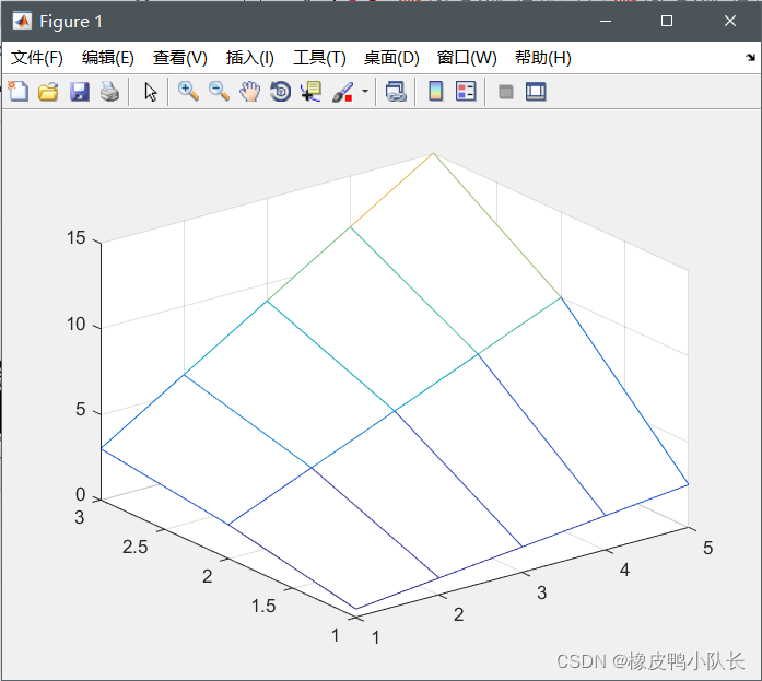
例:绘制空间曲线。
 >> x=2:6;
 >> y=(3:8)';
 >> [X,Y]=meshgrid(x,y);
>> Z=randn(size(X));
>> plot3(X,Y,Z);
>> grid on
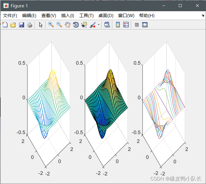
绘制三维曲面的mesh函数和surf函数
mesh(x,y,z,c)
surf(x,y,z,c)
c用于指定颜色。
例:绘制三维曲面图z = x e − x 2 − y 2 z=x e^{ -x^2-y^2}z=xe−x2−y2。
>> t=-2:0.2:2;
>> [X,Y]=meshgrid(t);
>> Z=X.*exp(-X.^2-Y.^2);
>> subplot(1,3,1)
>> mesh(X,Y,Z)
>> subplot(1,3,2)
>> surf(X,Y,Z);
>> subplot(1,3,3)
>> plot3(X,Y,Z);
>> grid on
mesh函数和surf函数的其他调用格式:
mesh(z,c)
surf(z,c)
当x、y省略时,z矩阵的第2维下标当作x轴坐标,z矩阵的第1维下标当作y轴坐标。
>> t=1:5;
>> z=[0.5*t;2*t;3*t];
>> mesh(z);
此外还有
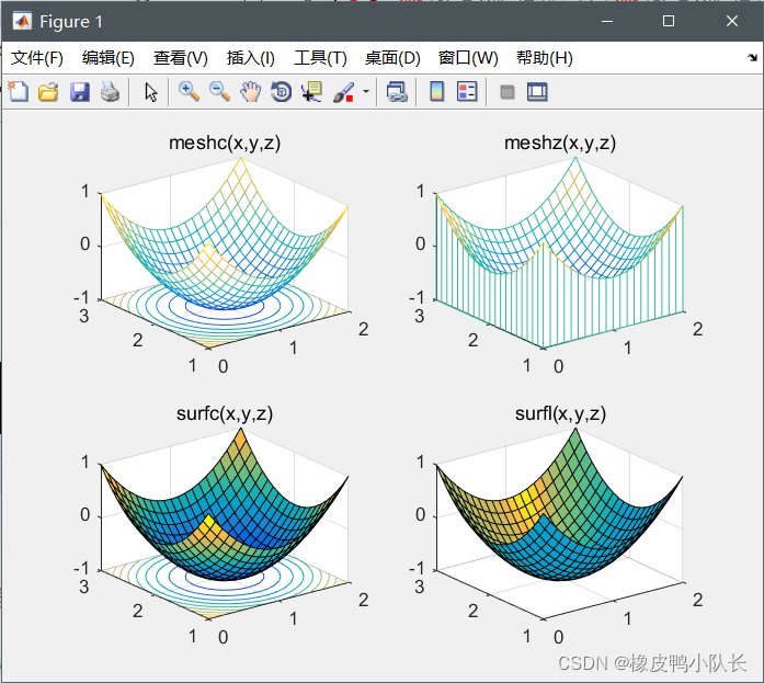
带等高线的三维网格曲面函数meshc
带底座的三维网格曲面函数meshz
具有等高线的曲面函数surfc
具有光照效果的曲面函数sufl
例:用4种方式绘制函数z = ( x + 1 ) 2 + ( y − 2 ) 2 − 1 z=(x+1)^2+(y-2)^2-1z=(x+1)2+(y−2)2−1的曲面图,其中x ∈ [ 0 , 2 ] , y ∈ [ 1 , 3 ] x\in[0,2],y\in[1,3]x∈[0,2],y∈[1,3]。
>> [x,y]=meshgrid(0:0.1:2,1:0.1:3);
>> z=(x-1).^2+(y-2).^2-1;
>> subplot(2,2,1)
>> meshc(x,y,z);title('meshc(x,y,z)')
>> subplot(2,2,2)
>> meshz(x,y,z);title('meshz(x,y,z)')
>> subplot(2,2,3)
>> surfc(x,y,z);title('surfc(x,y,z)')
>> subplot(2,2,4)
>> surfl(x,y,z);title('surfl(x,y,z)')
标准三维曲面
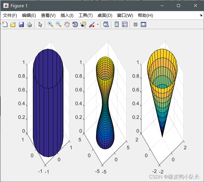
sphere函数
[x,y,z]=sphere(n)cylinder函数
[x,y,z]=cylinder(R,n)例:用cylinder函数分别绘制柱面、花瓶和圆锥面。
 >> subplot(1,3,1);
 >> [x,y,z]=cylinder;
 >> surf(x,y,z);
 >> subplot(1,3,2);
 >> t=linspace(0,2*pi,40);
 >> [x,y,z]=cylinder(2+cos(t),30);
 >> surf(x,y,z);
 >> subplot(1,3,3);
 >> [x,y,z]=cylinder(0:0.2:2,30);
 >> surf(x,y,z)
- peaks函数
多峰函数:
f ( x , y ) = 3 ( 1 − x 2 ) e − x 2 − ( y + 1 ) 2 − 10 x 5 − x 3 − y 5 e − x 2 − y 2 − 1 3 e − ( x + 1 ) 2 − y 2 f(x,y)=3(1-x^2)e^{-x^2-(y+1)^2}-10{\frac{x}{5}-x^3-y^5}e^{-x^2-y^2}-\frac{1}{3}e^{-(x+1)^2-y^2}f(x,y)=3(1−x2)e−x2−(y+1)2−105x−x3−y5e−x2−y2−31e−(x+1)2−y2
peaks函数的调用格式:
peaks(n)
peaks(V)
peaks(x,y)
peaks
>> p1=peaks(10);
>> p2=peaks;
>> p3=peaks(-3:0.2:3);
>> [x,y]=meshgrid(-2:0.1:2,0:0.1:5);
>> p4=peaks(x,y);
fmesh函数和fsurf函数
fmesh(funx,funy,funz,uvlims)
fsurf(funx,funy,funz,uvlims)
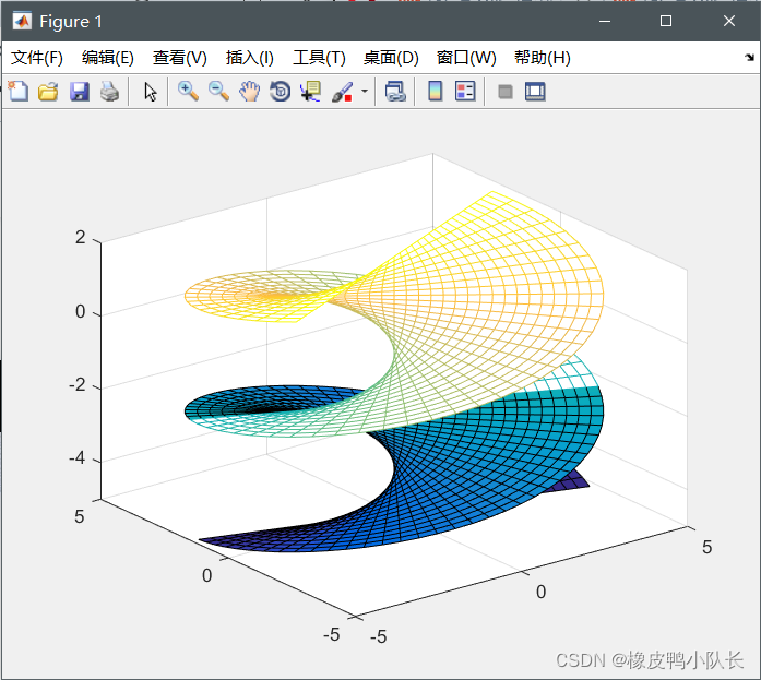
例:绘制螺旋曲面{ x = u s i n v y = − u c o s v , − 5 < u < 5 , − 5 < v < 2 z = v \begin{cases}x=usinv \\y=-ucosv,-5<u<5,-5<v<2\\z=v\end{cases}⎩⎪⎨⎪⎧x=usinvy=−ucosv,−5<u<5,−5<v<2z=v。
>> funx=@(u,v)u.*sin(v);
>> funy=@(u,v)-u.*cos(v);
>> funz=@(u,v)v;
>> fsurf(funx,funy,funz,[-5,5,-5,-2])
>> hold on
>> fmesh(funx,funy,funz,[-5,5,-2,2])
>> hold off
4.6图形修饰处理
渲染、烘托图形的表现效果,传达更多的信息。
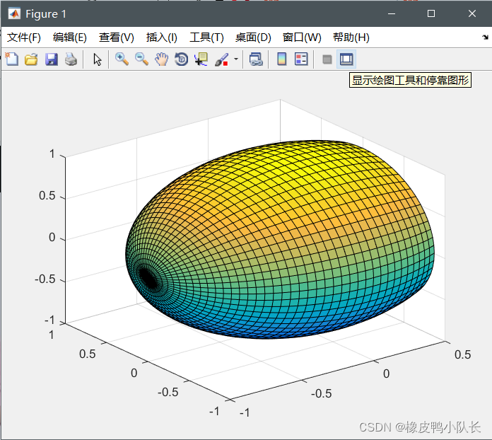
视点处理
view函数基本用法
view(az,el)
az为方位角,el为仰角。
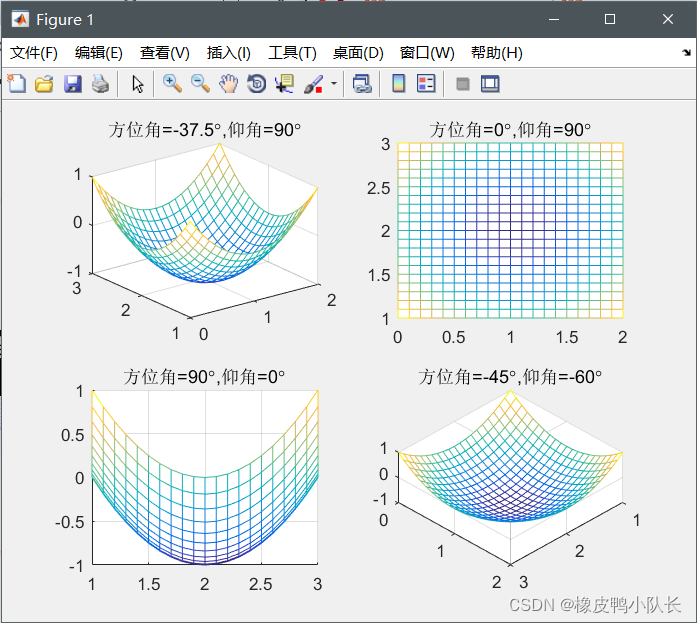
例:绘制函数z = ( x + 1 ) 2 + ( y − 2 ) 2 − 1 z=(x+1)^2+(y-2)^2-1z=(x+1)2+(y−2)2−1的曲面,并从不同视点展现曲面$。
	>> [x,y]=meshgrid(0:0.1:2,1:0.1:3);
	>> z=(x-1).^2+(y-2).^2-1;
	>> subplot(2,2,1);mesh(x,y,z)
	>> title('方位角=-37.5{\circ},仰角=90{\circ}')
	>> subplot(2,2,2);mesh(x,y,z)
	>> view(0,90);title('方位角=0{\circ},仰角=90{\circ}')
	>> subplot(2,2,3);mesh(x,y,z)
	>> view(90,0);title('方位角=90{\circ},仰角=0{\circ}')
	>> subplot(2,2,4);mesh(x,y,z)
	>> view(-45,-60);title('方位角=-45{\circ},仰角=-60{\circ}')
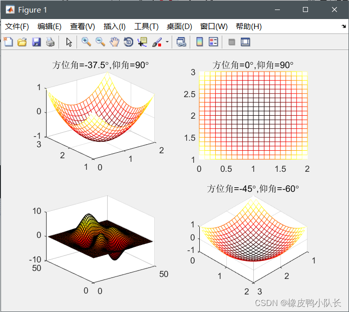
色彩处理
颜色的向量表示[R G B]
色图(Colormap)
色图矩阵
内建色图:冷暖色图、四季色图、灰度色图…
指定当前图形使用的色图
colormap cmapname
colormap(cmap)>> surf(peaks) >> colormap hot
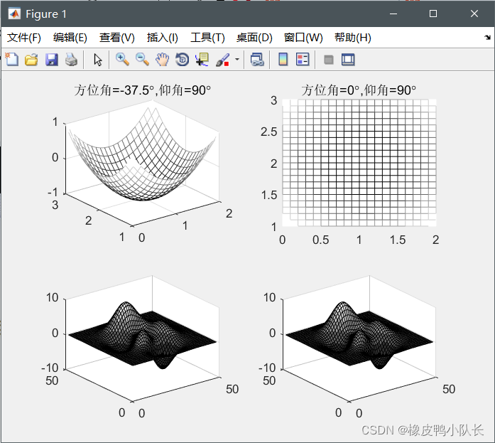
创建色图矩阵:
色图矩阵的每一行是RGB三元组。可以自定义色图矩阵,也可以调用MATLAB提供的函数来定义色图矩阵。
例:创建一个灰色系列色图矩阵。
>> c=[0,0.2,0.4,0.6,0.8,1]';
>> cmap=[c,c,c];
>> surf(peaks)
>> colormap(cmap)
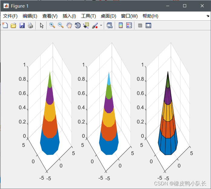
- 三维图形表面的着色
| shading faceted | shading flat | shasing interp |
|---|---|---|
| 将每个网格片用其高度对应的颜色进行着色,网格线是黑色。 | 将每个网格片用同一个的颜色进行着色,且网格线也用相应的颜色。 | 在网格片内采用颜色插值处理。 |
例:使用同一色图,以不同着色方式绘制圆锥体。
>> [x,y,z]=cylinder(pi:-pi/5:0,10);
>> colormap(lines);
>> subplot(1,3,1);
>> surf(x,y,z);shading flat
>> subplot(1,3,2);
>> surf(x,y,z);shading interp
>> subplot(1,3,3);
>> surf(x,y,z)
裁剪处理
将图形中需要裁剪部分对应的函数值设置为NaN。
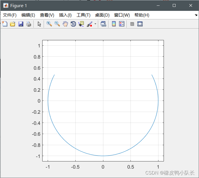
例:绘制3 / 4 3/43/4圆。
>> t = linspace(0,2*pi,100);
>> x = sin(t);
>> y = cos(t);
>> p = y>0.5;
>> y(p)=NaN;
>> plot(x,y)
>> axis([-1.1,1.1,-1.1,1.1])
>> axis square
>> grid on
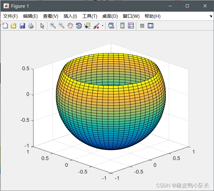
例:绘制3 / 4 3/43/4球面。
>> [X,Y,Z]=sphere(60);
>> p=Z>0.5;
>> Z(p)=NaN;
>> surf(X,Y,Z)
>> axis([-1,1,-1,1,-1,1])
>> axis equal
>> view(-45,20)
4.7交互式绘图工具
“绘图”选项卡

绘图工具
- 显示绘图工具
“显示绘图工具和停靠图形”按钮
命令行窗口输入命令
>>plottools
图形窗口绘图工具
