RIS components
This is a python project for RIS(reconfigurable intelligent surface) simulations.
related works
- My first paper Link to my paper / Pdf to my paper:
[1] X. Guo, Y. Chen and Y. Wang, “Learning-based Robust and Secure Transmission for Reconfigurable Intelligent Surface Aided Millimeter Wave UAV Communications,” in IEEE Wireless Communications Letters, doi: 10.1109/LWC.2021.3081464.
- DDPG structure
Refer to the following code on github:
\qquad a. tf-agent this is the easiest way the use the official RL(reinforcement learning) api.
\qquad b. open source RL api using tensorflow: (coming soon)
\qquad c. DDPG structure refters to [3](pdf). There has already been some works on the combination of the DDPG and the RIS [4](pdf)
- RIS simulation
Refer to the paper Link to this paper / Pdf to this paper. This paper provide a simulation code in matlab, we refer to this project to provide a python version.
[2] E. Basar and I. Yildirim, “SimRIS Channel Simulator for Reconfigurable Intelligent Surface-Empowered Communication Systems,” 2020 IEEE Latin-American Conference on Communications (LATINCOM), 2020, pp. 1-6, doi: 10.1109/LATINCOM50620.2020.9282349.
What this project aims ?
This project aims to redo the simulations shown in the paper below Link to this paper:
[3] Zhang, Zijian, et al. “Active RIS vs. Passive RIS: Which Will Prevail in 6G?.” arXiv preprint arXiv:2103.15154 (2021).
Specifically, in this project we will simulate the active RIS. And to maximum the universality, this project will provide modular simulation tool for RIS-aided system.
File structure
./cite
The cited paper for this project
./learning
The code to initialize the agents
\qquad ./learning/official
\qquad The offical RL agents api (tf-agent)
\qquad ./learning/custom
\qquad The third party open source RL agent api
RIS theory
this section mainly refers to [2] (SimRIS1.0) and [2.2] (SimRIS2.0).
RIS-Assisted LOS channels(SISO)
According to the plate scattering theory[2,(1)], the transmitted signal is captured by each RIS element, then rescattered to the medium in all directions. Focusing on he n nn-th RIS element, the captured power on it can be readily obtained as
P n R I S = P t G t G e T x λ 2 ( 4 π ) 2 a n 2 (1) P_{n}^{RIS}=\frac{P_tG_tG_e^{Tx}\lambda^2}{(4\pi)^2a_n^2} \tag{1}PnRIS=(4π)2an2PtGtGeTxλ2(1)
where P t P_tPt is the transmit power,G t G_tGt is the transmit antenna gain in the direction of the n nn-th RIS element (or the RIS in general), G e T x G_e^{Tx}GeTx is the gain of the corresponding RIS element in the direction of the transmitter (Tx), λ \lambdaλ is the wavelength, and a n a_nan is the distance between the transmitter and this element. The effective aperture of the n nn-th RIS element is G e T x λ 2 / ( 4 π ) G_{e}^{\mathrm{Tx}} \lambda^{2} /(4 \pi)GeTxλ2/(4π), and the power flux density incident on it given by P t G t / ( 4 π a n 2 ) P_{t} G_{t} /\left(4 \pi a_{n}^{2}\right)PtGt/(4πan2). Then the captured power is re-radiated to the medium with an efficiency factor ϵ \epsilonϵ, which in [2] is assumed to be unity.
The captured power at the receiver (Rx) is obtained as
P n R x = P n R I S G e R x G r λ 2 ( 4 π ) 2 b n 2 = P t G t G r G e T x G e R x λ 4 ( 4 π ) 4 a n 2 b n 2 (2) P_{n}^{\mathrm{Rx}}=\frac{P_{n}^{\mathrm{RIS}} G_{e}^{\mathrm{Rx}} G_{r} \lambda^{2}}{(4 \pi)^{2} b_{n}^{2}}=\frac{P_{t} G_{t} G_{r} G_{e}^{\mathrm{Tx}} G_{e}^{\mathrm{Rx}} \lambda^{4}}{(4 \pi)^{4} a_{n}^{2} b_{n}^{2}}\tag{2}PnRx=(4π)2bn2PnRISGeRxGrλ2=(4π)4an2bn2PtGtGrGeTxGeRxλ4(2)
where G r G_rGr is the receive antenna gain in the direction of the n nn-th RIS element and G e R x G_{e}^{\mathrm{Rx}}GeRx is the gain of the corresponding RIS element in the direction of the receiver. For the same scenario, let us consider the radar range equation given by
P r = P t G t G r λ 2 σ R C S ( 4 π ) 3 a n 2 b n 2 (3) P_{r}=\frac{P_{t} G_{t} G_{r} \lambda^{2} \sigma_{\mathrm{RCS}}}{(4 \pi)^{3} a_{n}^{2} b_{n}^{2}} \tag{3}Pr=(4π)3an2bn2PtGtGrλ2σRCS(3)
where σ R C S = 4 π A 2 / λ 2 \sigma_{\mathrm{RCS}}=4 \pi A^{2} / \lambda^{2}σRCS=4πA2/λ2 is the radar cross section (RCS, in m 2 m^2m2) of the RIS element with A AA being its physical area. (2) and (3) are actually the same, given σ R C S = λ 2 G e 2 / 4 π \sigma_{RCS} =\lambda^{2} G_{e}^{2} / 4 \piσRCS=λ2Ge2/4π.
Let’s assum the parameters as:
| Parameter |
|---|
| P t = 0 dBW P_t = 0\ \text{dBW}Pt=0 dBW |
| G t = G r = 1 ( 0 dBi ) G_t= G_r = 1\ (0\ \text{dBi})Gt=Gr=1 (0 dBi) |
| $ G_{e}=\pi\ (5\ \mathrm{dBi})$ (Reference)[2-9] |
Then the received power through n nn-th RIS element is:
P n R x = G e 2 λ 4 ( 4 π ) 4 a n 2 b n 2 (4) P_{n}^{\mathrm{Rx}}=\frac{G_{e}^{2} \lambda^{4}}{(4 \pi)^{4} a_{n}^{2} b_{n}^{2}}\tag{4}PnRx=(4π)4an2bn2Ge2λ4(4)
The total path loss is:
L n = L n , 1 × L n , 2 = G e λ 2 ( 4 π ) 2 a n 2 × G e λ 2 ( 4 π ) 2 b n 2 (5) L_{n}=L_{n, 1} \times L_{n, 2}=\frac{G_{e} \lambda^{2}}{(4 \pi)^{2} a_{n}^{2}} \times \frac{G_{e} \lambda^{2}}{(4 \pi)^{2} b_{n}^{2}}\tag{5}Ln=Ln,1×Ln,2=(4π)2an2Geλ2×(4π)2bn2Geλ2(5)
In general, the received signal at the receiver is:
y = ( ∑ n = 1 N P n R x ( α n e j ϕ n ) e − j k ( a n + b n ) ) x (6) y=\left(\sum_{n=1}^{N} \sqrt{P_{n}^{\mathrm{Rx}}}\left(\alpha_{n} e^{j \phi_{n}}\right) e^{-j k\left(a_{n}+b_{n}\right)}\right) x\tag{6}y=(n=1∑NPnRx(αnejϕn)e−jk(an+bn))x(6)
Where α n \alpha_nαn and $ \phi_n$ respectively stand for controllable magnitude and phase response of the nth element, k = 2 π / λ k=2 \pi / \lambdak=2π/λ is the wave number, and x xx is the transmitted signal. . One can easily observe from (6) that the received signal power can be maximized by adjusting RIS element phases as ϕ n = k ( a n + b n ) \phi_{n}=k\left(a_{n}+b_{n}\right)ϕn=k(an+bn). Finally, it is worth noting that the direct link between Tx and Rx can be incorporated into the model by
y = ( ∑ n = 1 N P n R x ( α n e j ϕ n ) e − j k ( a n + b n ) + P T − R e − j k d T − R ) x (7) y=\left(\sum_{n=1}^{N} \sqrt{P_{n}^{\mathrm{Rx}}}\left(\alpha_{n} e^{j \phi_{n}}\right) e^{-j k\left(a_{n}+b_{n}\right)}+\sqrt{P_{\mathrm{T}-\mathrm{R}}} e^{-j k d_{\mathrm{T-R}}}\right) x\tag{7}y=(n=1∑NPnRx(αnejϕn)e−jk(an+bn)+PT−Re−jkdT−R)x(7)
Where P T − R = λ 2 / ( 4 π d T − R ) 2 P_{\mathrm{T}-\mathrm{R}}=\lambda^{2} /\left(4 \pi d_{\mathrm{T}-\mathrm{R}}\right)^{2}PT−R=λ2/(4πdT−R)2 and d T − R d_{T-R}dT−R being the Tx-Rx distance.
RIS-Assisted channels(MIMO)[2.2]
| Parameter | Meanings | Dimension |
|---|---|---|
| N t N_{t}Nt | transmiter antennas number | R {\mathbb R}R |
| N r N_{r}Nr | receiver antennas number | R {\mathbb R}R |
| C \mathbf{C}C | End-to-end channel matrix | C N r × N t {\mathbb C}^{N_r \times N_t}CNr×Nt |
| D {\mathbf D}D | Direct channel matrix | C N r × N t {\mathbb C}^{N_r \times N_t}CNr×Nt |
| H {\bf H}H | The matrix of channel coefficients between the Tx and the RIS | C N × N t {\mathbb C}^{N \times N_t}CN×Nt |
| G {\bf G}G | The matrix of channel coefficients between the Tx and the RIS | C N r × N \mathbb{C}^{N_{r} \times N}CNr×N |
| Φ {\bf \Phi}Φ | The response of the RIS array | C N × N \mathbb{C}^{N \times N}CN×N |
C = G Φ H + D \mathbf{C}=\mathbf{G} \mathbf{\Phi} \mathbf{H}+\mathbf{D}C=GΦH+D
R = log 2 det ( I N r + P t σ 2 C H C ) b i t / s e c / H z R=\log _{2} \operatorname{det}\left(\mathbf{I}_{N_{r}}+\frac{P_{t}}{\sigma^{2}} \mathbf{C}^{H} \mathbf{C}\right) \mathrm{bit} / \mathrm{sec} / \mathrm{Hz}R=log2det(INr+σ2PtCHC)bit/sec/Hz
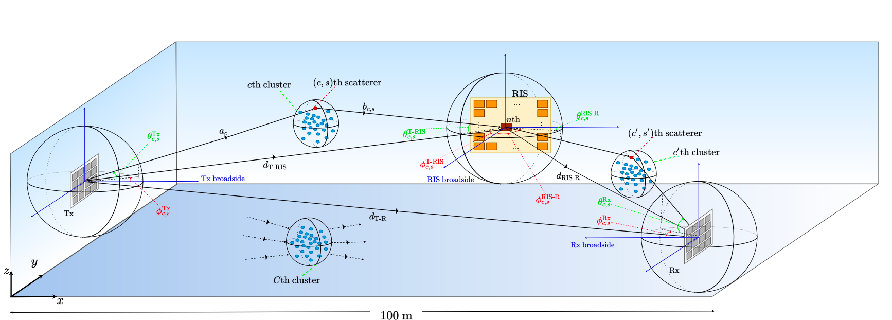
channel generation
The detailed channel modeling can be seen in 3GPP 38.901 [5].
The basic idea to model the mmWave channel is to consider the channel under SISO senirio and then by multiplexing the array response, we can get the result of a mmWave channel under MIMO senirio.
The detailed SISO channel model can be found in [6]
path loss
cluster and sub-ray
According to [6], the scatter paths are caused by the interacting objects (IOs) between the transceivers.
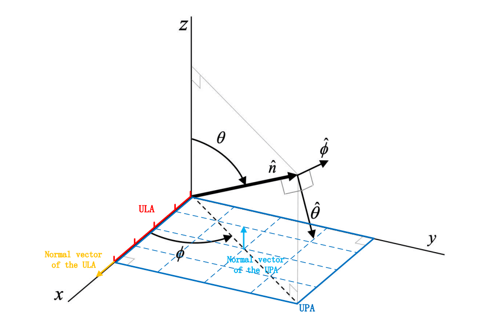
array response
the defination of the AoA and AoD is shown below:
Others
coding platform: Win10 pro, anaconda3
nvidia driver: 466.47
cuda version: cuda_11.1.1_456.81_win10
cuddn version: cudnn-11.2-windows-x64-v8.1.1.33
tensorflow version: 2.4.0
python version: 3.8.10
Cited papers
[1](pdf) X. Guo, Y. Chen and Y. Wang, “Learning-based Robust and Secure Transmission for Reconfigurable Intelligent Surface Aided Millimeter Wave UAV Communications,” in IEEE Wireless Communications Letters, doi: 10.1109/LWC.2021.3081464.
[2.0] E. Basar and I. Yildirim, “SimRIS Channel Simulator for Reconfigurable Intelligent Surface-Empowered Communication Systems,” 2020 IEEE Latin-American Conference on Communications (LATINCOM), 2020, pp. 1-6, doi: 10.1109/LATINCOM50620.2020.9282349. note this and [2.1] is corresponding to the SimRIS1.0 which considers the SISO system
[2.1] E. Basar, I. Yildirim, “Indoor and Outdoor Physical Channel Modeling and Efficient Positioning for Reconfigurable Intelligent Surfaces in mmWave Bands“, ArXiv:2006.02240, May 2020
[2.2] E. Basar, I. Yildirim, “SimRIS Channel Simulator for Reconfigurable Intelligent Surfaces in Future Wireless Networks”, ArXiv:2008.01448, Aug. 2020.this is corresponding to the SimRIS2.0 which considers the MIMO system
[3](pdf) Lillicrap, Timothy P., et al. “Continuous control with deep reinforcement learning.” arXiv preprint arXiv:1509.02971 (2015).
[4](pdf) Wang, Liang, et al. “Joint trajectory and passive beamforming design for intelligent reflecting surface-aided UAV communications: A deep reinforcement learning approach.” arXiv preprint arXiv:2007.08380 (2020).
[5] 3GPP, “Study on channel model for frequencies from 0.5 to 100 GHz,”
3rd Generation Partnership Project (3GPP), Technical Specification (TS)
38.901, 01 2020, version 16.1.0.
[6] E. Basar and I. Yildirim, “Indoor and outdoor physical channel
modeling and efficient positioning for reconfigurable intelligent
surfaces in mmWave bands,” Aug. 2020. [Online]. Available:
https://arxiv.org/abs/2006.02240