pca降维分类_降维-PCA是否可以改善分类模型的性能？

什么是PCA？ (What is PCA?)

Principal Component Analysis (PCA) is a common feature extraction technique in data science that employs matrix factorization to reduce the dimensionality of data into lower space.

主成分分析(PCA)是数据科学中的一种常见特征提取技术，该技术采用矩阵分解来减少数据进入较低空间的维数。

In real-world datasets, there are often too many features in the data. The higher the number of features harder it is to visualize the data and work on it. Sometimes most of the features are correlated, and hence redundant. Hence feature extraction comes into play.

在现实世界的数据集中，数据中通常有太多特征。 功能数量越多，就越难以可视化数据并对其进行处理。 有时大多数功能是相关的，因此是多余的。 因此，特征提取开始起作用。

关于数据： (About the Data:)

The dataset used in this article is Ionosphere Dataset from the UCI machine learning repository. It is a binary class classification problem. There are 351 observations with 34 features.

本文中使用的数据集是UCI机器学习存储库中的Ionosphere数据集 。 这是一个二进制类分类问题。 有351个观测结果，具有34个特征。

准备数据集： (Preparing the Dataset:)

• Importing necessary libraries and reading the dataset
  导入必要的库并读取数据集
• Preprocessing of dataset
  数据集的预处理
• Standardization
  标准化

import pandas as pd
import numpy as np
from sklearn.preprocessing import StandardScaler
rom sklearn.model_selection import train_test_split


data = pd.read_csv("ionosphere.csv", header=None)


X = data.iloc[:,:-1]
y = data.iloc[:,-1]


y = [1 if x=='g' else 0 for x in y]
y = np.reshape(y, (len(y), 1))


X_train, X_test, y_train, y_test = train_test_split(X, y, test_size=0.3)


std = StandardScaler()
X_train_std = std.fit_transform(X_train)
X_test_std = std.transform(X_test)


y_train = np.reshape(y_train, (y_train.shape[0]))
y_test = np.reshape(y_test, (y_test.shape[0]))


y_train = y_train.astype('int')
y_test = y_test.astype('int')

使用所有34个功能的Logistic回归ML模型： (Logistic Regression ML model using all 34 features:)

The training data has 34 features.

训练数据具有34个特征。

• After preprocessing of data, training data is trained using Logistic Regression algorithm for binary class classification
  在对数据进行预处理之后，使用Logistic回归算法对训练数据进行训练，以进行二分类分类
• Finetuning Logistic Regression model to find the best parameters
  微调Logistic回归模型以找到最佳参数
• Compute training and test accuracy and f1 score.
  计算训练和测试的准确性以及f1分数。

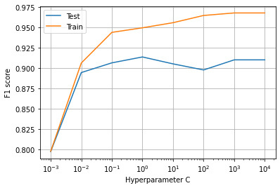
• Training an LR model using 34 features for c=10**0
  使用c = 10 ** 0的34个特征训练LR模型
• Compute training and test accuracy and f1 score
  计算训练和测试准确性以及f1分数

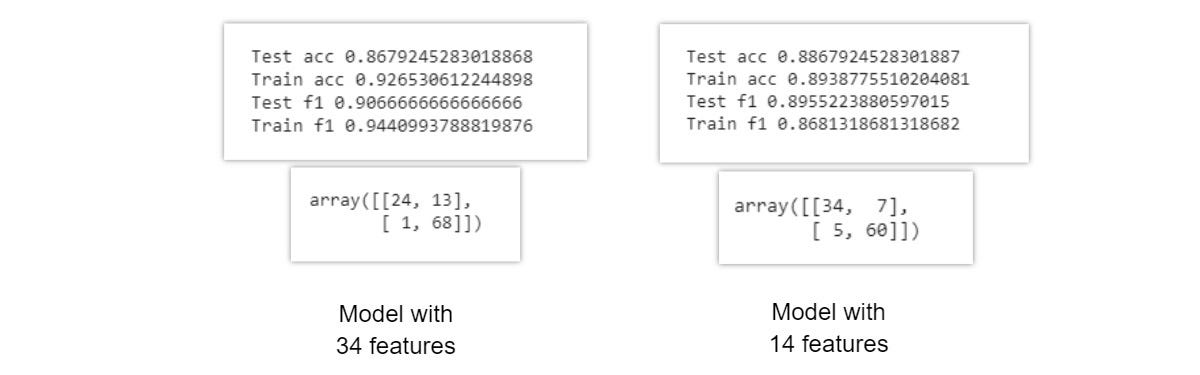
Results obtained by training the entire “X_train” data having 34 features,

通过训练具有34个特征的整个“ X_train”数据获得的结果，

the test f1-score is 0.90, as 14 values are misclassified as observed in the confusion matrix.

测试f1-分数为0.90，因为混淆矩阵中观察到14个值被错误分类。

import matplotlib.pyplot as plt
from sklearn.linear_model import LogisticRegression
from sklearn.metrics import *


C = [10**-3, 10**-2, 10**-1, 10**0, 10**1, 10**2, 10**3, 10**4]
f1_tr = []
f1_te = []
for c in C:
  model = LogisticRegression(C=c)
  model.fit(X_train_std, y_train)
  f1_te.append(f1_score(model.predict(X_test_std), y_test))
  f1_tr.append(f1_score(model.predict(X_train_std), y_train))
  print(c, f1_score(model.predict(X_test_std), y_test))
  
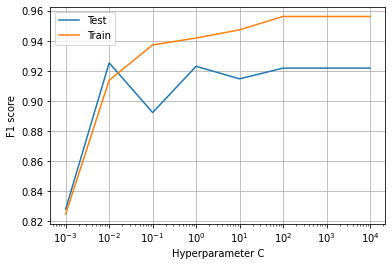
plt.plot(C, f1_te, label="Test")
plt.plot(C, f1_tr, label="Train")
plt.xlabel("Hyperparameter C")
plt.ylabel("F1 score")
plt.xscale("log")
plt.legend()
plt.grid()
plt.show()


model = LogisticRegression(C=10**0)
model.fit(X_train_std, y_train)


y_pred_te = model.predict(X_test_std)
y_pred_tr = model.predict(X_train_std)


print("Test acc", accuracy_score(y_test, y_pred_te))
print("Train acc", accuracy_score(y_train, y_pred_tr))


print("Test f1", f1_score(y_test, y_pred_te))
print("Train f1", f1_score(y_train, y_pred_tr))


print(confusion_matrix(y_test, y_pred_te))

使用PCA提取特征： (Feature Extraction using PCA:)

To extract features from the dataset using the PCA technique, firstly we need to find the percentage of variance explained as dimensionality decreases.

为了使用PCA技术从数据集中提取特征，首先我们需要找到因维数减少而解释的方差百分比。

Notations,λ: eigenvalue
d: number of dimension of original datasetk: number of dimensions of new feature space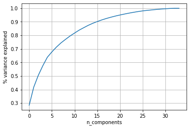

• From the above plot, it is observed that for 15 dimensions the percentage of variance explained is 90%. This means we are preserving 90% of variance by projecting higher dimensionality (34) into lower space (15).
  从上图可以看出，对于15个维度，解释的差异百分比为90％。 这意味着我们通过将较高的尺寸(34)投影到较低的空间(15)中来保留90％的方差。

from sklearn.decomposition import PCA


pca = PCA(n_components=34)
pca_data = pca.fit_transform(X_train_std)


percent_var_explained = pca.explained_variance_/(np.sum(pca.explained_variance_))
cumm_var_explained = np.cumsum(percent_var_explained)


plt.plot(cumm_var_explained)
plt.grid()
plt.xlabel("n_components")
plt.ylabel("% variance explained")
plt.show()


pca = PCA(n_components=15)
pca_train_data = pca.fit_transform(X_train_std)
pca_test_data = pca.transform(X_test_std)

使用PCA的前15个功能来训练Logistic回归ML模型： (Training Logistic Regression ML model using top 15 features from PCA:)

Now the training data after PCA dimensionality reduction has 15 features.

现在，PCA降维后的训练数据具有15个特征。

• After preprocessing of data, training data is trained using Logistic Regression algorithm for binary class classification
  在对数据进行预处理之后，使用Logistic回归算法对训练数据进行训练，以进行二分类分类
• Finetuning Logistic Regression model to find the best parameters
  微调Logistic回归模型以找到最佳参数
• Compute training and test accuracy and f1 score.
  计算训练和测试的准确性以及f1分数。

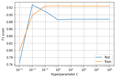
• Training an LR model using 15 feature for c=10**0
  使用c = 10 ** 0的15个特征训练LR模型
• Compute training and test accuracy and f1 score
  计算训练和测试准确性以及f1分数

Results obtained by training the PCA data with 15 features,

通过训练具有15种特征的PCA数据获得的结果，

the test f1-score is 0.896, as 12 values are misclassified as observed in the confusion matrix.

测试f1-分数为0.896，因为在混淆矩阵中观察到12个值被错误分类。

比较以上两个模型的结果： (Comparing the results of the above two models:)

import matplotlib.pyplot as plt
from sklearn.linear_model import LogisticRegression
from sklearn.metrics import *


C = [10**-3, 10**-2, 10**-1, 10**0, 10**1, 10**2, 10**3, 10**4]
f1_tr = []
f1_te = []
for c in C:
  model = LogisticRegression(C=c)
  model.fit(X_train_std, y_train)
  f1_te.append(f1_score(model.predict(X_test_std), y_test))
  f1_tr.append(f1_score(model.predict(X_train_std), y_train))
  print(c, f1_score(model.predict(X_test_std), y_test))
  
plt.plot(C, f1_te, label="Test")
plt.plot(C, f1_tr, label="Train")
plt.xlabel("Hyperparameter C")
plt.ylabel("F1 score")
plt.xscale("log")
plt.legend()
plt.grid()
plt.show()


model = LogisticRegression(C=10**0)
model.fit(X_train_std, y_train)


y_pred_te = model.predict(X_test_std)
y_pred_tr = model.predict(X_train_std)


print("Test acc", accuracy_score(y_test, y_pred_te))
print("Train acc", accuracy_score(y_train, y_pred_tr))


print("Test f1", f1_score(y_test, y_pred_te))
print("Train f1", f1_score(y_train, y_pred_tr))


print(confusion_matrix(y_test, y_pred_te))

使用原始数据+来自PCA的数据来训练LR模型： (Training LR model using original data + data from PCA:)

After concatenating original data with 34 features and PCA data with 15 features, we form a dataset of 49 features.

将具有34个特征的原始数据与具有15个特征的PCA数据连接起来后，我们形成了49个特征的数据集。

• After preprocessing of data, training data is trained using Logistic Regression algorithm for binary class classification
  在对数据进行预处理之后，使用Logistic回归算法对训练数据进行训练，以进行二分类分类
• Finetuning Logistic Regression model to find the best parameters
  微调Logistic回归模型以找到最佳参数
• Compute training and test accuracy and f1 score.
  计算训练和测试的准确性以及f1分数。

• Training an LR model using 15 feature for c=10**0
  使用c = 10 ** 0的15个特征训练LR模型
• Compute training and test accuracy and f1 score
  计算训练和测试准确性以及f1分数

concat_train_data = np.concatenate((X_train_std, pca_train_data), 1)
concat_test_data = np.concatenate((X_test_std, pca_test_data), 1)


C = [10**-3, 10**-2, 10**-1, 10**0, 10**1, 10**2, 10**3, 10**4]
f1_tr = []
f1_te = []
for c in C:
  model = LogisticRegression(C=c)
  model.fit(concat_train_data, y_train)
  f1_te.append(f1_score(model.predict(concat_test_data), y_test))
  f1_tr.append(f1_score(model.predict(concat_train_data), y_train))


plt.plot(C, f1_te, label="Test")
plt.plot(C, f1_tr, label="Train")
plt.xlabel("Hyperparameter C")
plt.ylabel("F1 score")
plt.xscale("log")
plt.legend()
plt.grid()
plt.show()


model = LogisticRegression(C=10**0)
model.fit(concat_train_data, y_train)


y_pred_te = model.predict(concat_test_data)
y_pred_tr = model.predict(concat_train_data)


print("Test acc", accuracy_score(y_test, y_pred_te))
print("Train acc", accuracy_score(y_train, y_pred_tr))


print("Test f1", precision_score(y_test, y_pred_te))
print("Train f1", precision_score(y_train, y_pred_tr))


print(confusion_matrix(y_test, y_pred_te))

以上结果总结： (Conclusions from the above results:)

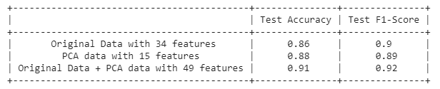
From the above pretty table, we can observe that,

从上面的漂亮表格中，我们可以观察到，

• An LR model trained using the raw preprocessed dataset with 34 features, we get an F1-score of 90%.
  使用具有34个特征的原始预处理数据集训练的LR模型，我们得到的F1得分为90％。
• An LR model trained only with extracted 15 features using PCA, we get an F1-score of 89%.
  一个仅使用PCA提取15个特征进行训练的LR模型，我们的F1得分为89％。
• An LR model trained with a combination of the above two data, we get an F1-score of 92%.
  通过结合以上两个数据训练的LR模型，我们的F1得分为92％。

Let’s observe the change in Confusion Matrix results for the above-mentioned 3 models.

让我们观察一下上述3个模型的混淆矩阵结果的变化。

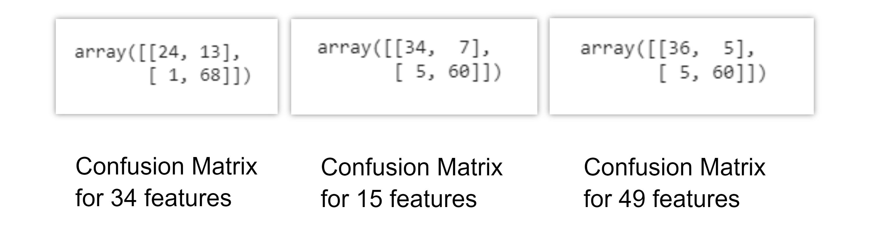
Hence we conclude that using only PCA extracted features with only 50% of numbers of features from original data we get 1% less F1-score. But if we combine both data we improve the metric of 2% to get the final F1-score of 91%.

因此，我们得出的结论是，仅使用PCA提取的特征，而原始数据仅占特征数目的50％，则我们的F1分数就会减少1％。 但是，如果我们将这两个数据结合起来，我们的指标将提高2％，从而使最终的F1得分达到91％。

Click below to get code:

点击下面获取代码：

Thank You for Reading

谢谢您的阅读