神经网络 tensorflow ：损失函数

基础理论

交叉熵

参考：https://zhuanlan.zhihu.com/p/35709485
常用于分类问题，但是也可以用于回归问题

tensorFlow中的损失函数

BinaryCrosstropy

计算真实标签和预测标签之间的交叉熵损失。
当只有两个标签类别（假定为0和1）时，请使用此交叉熵损失。对于每个示例，每个预测应该有一个浮点值。

tf.keras.losses.BinaryCrossentropy(
    from_logits=False, label_smoothing=0, reduction=losses_utils.ReductionV2.AUTO,
    name='binary_crossentropy'
)

y_true = [[0., 1.], [0., 0.]]
y_pred = [[0.6, 0.4], [0.4, 0.6]]
# Using 'auto'/'sum_over_batch_size' reduction type.
bce = tf.keras.losses.BinaryCrossentropy()
bce(y_true, y_pred).numpy()

CategoricalCrossentropy

计算标签和预测之间的交叉熵损失。
当有两个或多个标签类别时，请使用此交叉熵损失函数。我们希望标签以one_hot表示形式提供。如果要以整数形式提供标签，请使用SparseCategoricalCrossentropy损失。

tf.keras.losses.CategoricalCrossentropy(
    from_logits=False, label_smoothing=0, reduction=losses_utils.ReductionV2.AUTO,
    name='categorical_crossentropy'
)

y_true = [[0, 1, 0], [0, 0, 1]]
y_pred = [[0.05, 0.95, 0], [0.1, 0.8, 0.1]]
# Using 'auto'/'sum_over_batch_size' reduction type.
cce = tf.keras.losses.CategoricalCrossentropy()
cce(y_true, y_pred).numpy()

CosineSimilarity

直接计算l2范数的差别
loss = -sum(l2_norm(y_true) * l2_norm(y_pred))

y_true = [[0., 1.], [1., 1.]]
y_pred = [[1., 0.], [1., 1.]]
# Using 'auto'/'sum_over_batch_size' reduction type.
cosine_loss = tf.keras.losses.CosineSimilarity(axis=1)
# l2_norm(y_true) = [[0., 1.], [1./1.414], 1./1.414]]]
# l2_norm(y_pred) = [[1., 0.], [1./1.414], 1./1.414]]]
# l2_norm(y_true) . l2_norm(y_pred) = [[0., 0.], [0.5, 0.5]]
# loss = mean(sum(l2_norm(y_true) . l2_norm(y_pred), axis=1))
#       = -((0. + 0.) +  (0.5 + 0.5)) / 2
cosine_loss(y_true, y_pred).numpy()

Hinge

loss = maximum(1 - y_true * y_pred, 0)

y_true = [[0., 1.], [0., 0.]]
y_pred = [[0.6, 0.4], [0.4, 0.6]]
# Using 'auto'/'sum_over_batch_size' reduction type.
h = tf.keras.losses.Hinge()
h(y_true, y_pred).numpy()

Huber

结合了均方误差和平均绝对值误差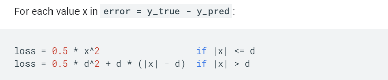

tf.keras.losses.Huber(
    delta=1.0, reduction=losses_utils.ReductionV2.AUTO, name='huber_loss'
)

y_true = [[0, 1], [0, 0]]
y_pred = [[0.6, 0.4], [0.4, 0.6]]
# Using 'auto'/'sum_over_batch_size' reduction type.
h = tf.keras.losses.Huber()
h(y_true, y_pred).numpy()

KLDivergence

相对熵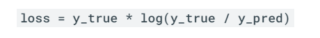

y_true = [[0, 1], [0, 0]]
y_pred = [[0.6, 0.4], [0.4, 0.6]]
# Using 'auto'/'sum_over_batch_size' reduction type.
kl = tf.keras.losses.KLDivergence()
kl(y_true, y_pred).numpy()

LogCosh

y_true = [[0., 1.], [0., 0.]]
y_pred = [[1., 1.], [0., 0.]]
# Using 'auto'/'sum_over_batch_size' reduction type.
l = tf.keras.losses.LogCosh()
l(y_true, y_pred).numpy()

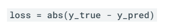
MeanAbsoluteError

y_true = [[0., 1.], [0., 0.]]
y_pred = [[1., 1.], [1., 0.]]
# Using 'auto'/'sum_over_batch_size' reduction type.
mae = tf.keras.losses.MeanAbsoluteError()
mae(y_true, y_pred).numpy()

MeanAbsolutePercentageError

y_true = [[2., 1.], [2., 3.]]
y_pred = [[1., 1.], [1., 0.]]
# Using 'auto'/'sum_over_batch_size' reduction type.
mape = tf.keras.losses.MeanAbsolutePercentageError()
mape(y_true, y_pred).numpy()

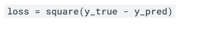
MeanSquaredError

y_true = [[0., 1.], [0., 0.]]
y_pred = [[1., 1.], [1., 0.]]
# Using 'auto'/'sum_over_batch_size' reduction type.
mse = tf.keras.losses.MeanSquaredError()
mse(y_true, y_pred).numpy()

MeanSquaredLogarithmicError

y_true = [[0., 1.], [0., 0.]]
y_pred = [[1., 1.], [1., 0.]]
# Using 'auto'/'sum_over_batch_size' reduction type.
msle = tf.keras.losses.MeanSquaredLogarithmicError()
msle(y_true, y_pred).numpy()

Poisson

y_true = [[0., 1.], [0., 0.]]
y_pred = [[1., 1.], [0., 0.]]
# Using 'auto'/'sum_over_batch_size' reduction type.
p = tf.keras.losses.Poisson()
p(y_true, y_pred).numpy()

SquaredHinge

y_true = [[0., 1.], [0., 0.]]
y_pred = [[0.6, 0.4], [0.4, 0.6]]
# Using 'auto'/'sum_over_batch_size' reduction type.
h = tf.keras.losses.SquaredHinge()
h(y_true, y_pred).numpy()