1997年提出的
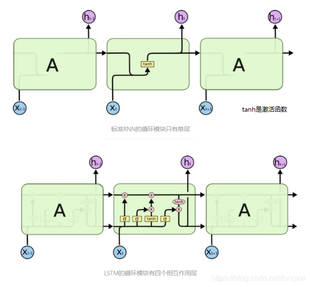
LSTM是一种特殊的RNN,表现突出。很好地解决了训练RNN过程中的各种问题,在几乎各类问题中都展现出远好于Vanilla RNN的表现
LSTM 和基本的 RNN 是一样的, 他的参数也是相同的
长期依赖(Long-Term Dependencies)问题
长期依赖(Long-Term Dependencies)问题 也就是我们在RNN中说的,由于梯度弥散和梯度爆炸,RNN不具备长期记忆,而只具备短期记忆的问题
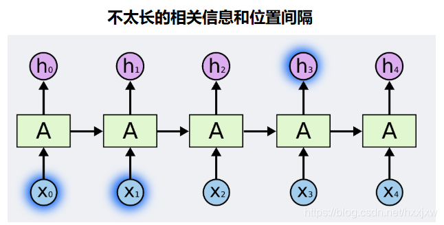
有时候,我们仅仅需要知道先前的信息来执行当前的任务。例如,我们有一个语言模型用来基于先前的词来预测下一个词。如果我们试着预测 “the clouds are in the sky” 最后的词,我们并不需要任何其他的上下文 —— 因此下一个词很显然就应该是 sky。在这样的场景中,相关的信息和预测的词位置之间的间隔是非常小的,RNN 可以学会使用先前的信息。
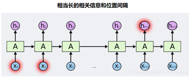
但是同样会有一些更加复杂的场景。假设我们试着去预测“I grew up in France... I speak fluent French”最后的词。当前的信息建议下一个词可能是一种语言的名字,但是如果我们需要弄清楚是什么语言,我们是需要先前提到的离当前位置很远的 France 的上下文的。这说明相关信息和当前预测位置之间的间隔就肯定变得相当的大。
不幸的是,在这个间隔不断增大时,RNN 会丧失学习到连接如此远的信息的能力。
但是,LSTM能够解决这个问题!
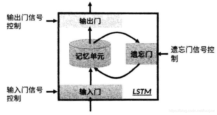
LSTM —— 长短期记忆网络LSTM是一种特殊的RNN,主要通过三个门控逻辑实现(遗忘、输入、输出)。它的提出就是为了解决长序列训练过程中的梯度消失和梯度爆炸问题
其核心关键在于:
- 提出了门机制:遗忘门、输入门、输出门;
- 细胞状态:在RNN中只有隐藏状态的传播,而在LSTM中,引入了细胞状态。
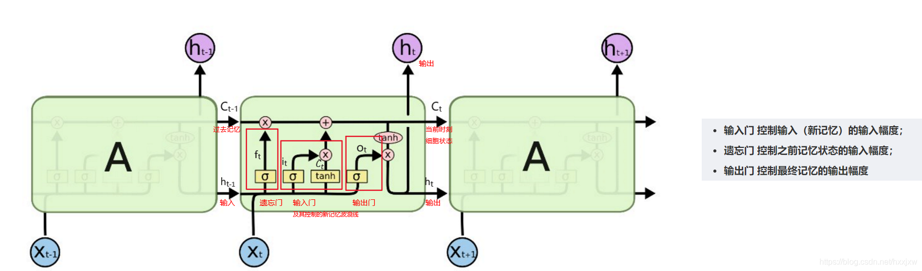
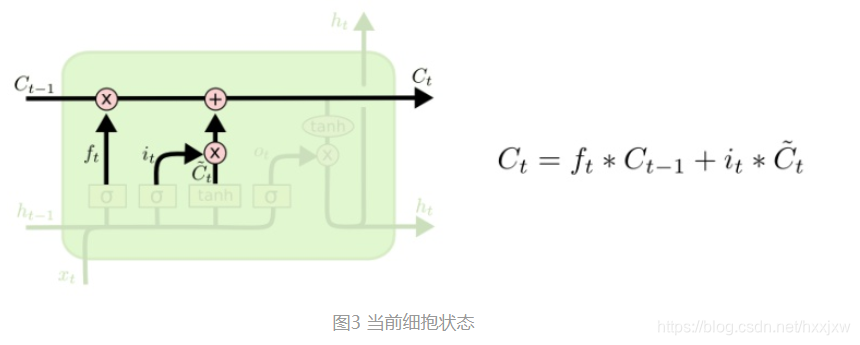
如图所示,其中相较于传统RNN单元,LSTM不仅有hidden-state h,还有细胞状态cell-state C. 而其中
sigmoid 则被称为门gate(值为0代表不通过任何信息,值为1代表全部通过),通过乘运算与和运算实现数据的合并与过滤。每个LSTM单元的输出有两个,一个是下面的ht,一个是上面的ct。ct的存在能很好地抑制梯度消失和梯度爆炸问题。
LSTM的核心
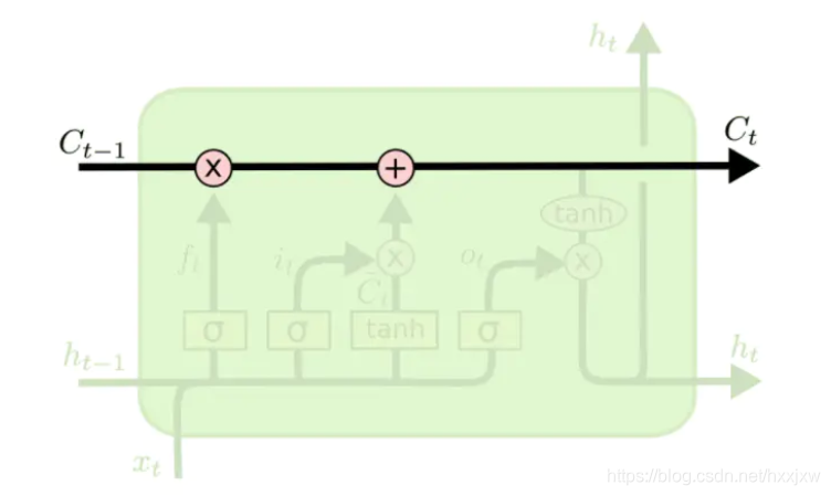
LSTM的核心是细胞状态,表示细胞状态的这条线水平的穿过图的顶部。
细胞的状态类似于输送带,细胞的状态在整个链上运行,只有一些小的线性操作作用其上,信息很容易保持不变的流过整个链。
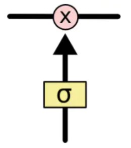
LSTM确实具有删除或添加信息到细胞状态的能力,这个能力是由被称为门(Gate)的结构所赋予的。
门(Gate)是一种可选地让信息通过的方式。 它由一个Sigmoid神经网络层和一个点乘法运算组成。
Sigmoid神经网络层输出0和1之间的数字,这个数字描述每个组件有多少信息可以通过, 0表示不通过任何信息,1表示全部通过
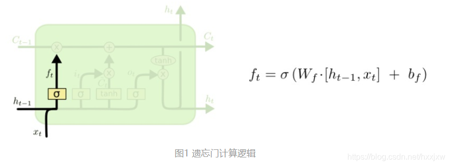
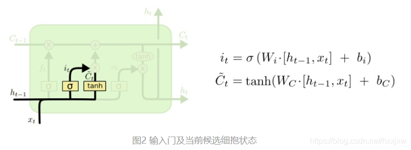
LSTM的遗忘、输入、输出三个门,用于保护和控制细胞的状态。
LSTM分层结构
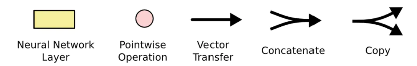
LSTM结构图中每一行都带有一个向量,该向量从一个节点输出到其他节点的输入。 粉红色圆圈表示点向运算,如向量加法、点乘,而黄色框是学习神经网络层。 线的合并表示连接,而线的交叉表示其内容正在复制,副本将转到不同的位置。
为什么LSTM能解决梯度弥散
原始RNN的ht-1到ht没有一个直通的通道,都必须经过Whh,才造成了Whh^k的情形
而LSTM有了一个memory直通的通道,有点类似于Resnet
另外LSTM之中采用了sigmoid作激活函数
当LSTM网络很深时且使用tanh作为激活函数,可能会引起梯度消失的问题。
Pytorch LSTM
Pytorch — LSTM_hxxjxw的博客-CSDN博客
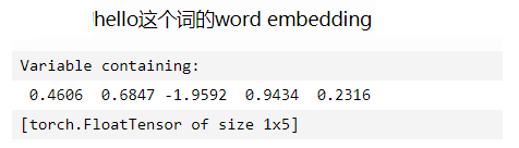
Word Embedding 词嵌入
词嵌入就是将文字转换成数字向量,因为计算机认识数字,不认识文字
词嵌入向量的意思也可以理解成:词在神经网络中的向量表示
例如,
padding_idx
自然语言中使用批处理时候, 每个句子的长度并不一定是等长的, 这时候就需要对较短的句子进行padding
......
LSTM进行句子单词词性预测
输入数据是句子和对句子中的字的词性的标签,给出新句子让网络能够预测句子中词的词性
RNN对文本等进行处理的时候,都是先将文本/字符转成数字向量,由数字向量输入LSTM等模型中,不会直接处理字符的
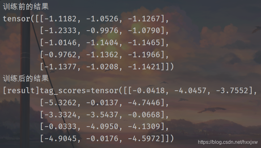
import torch
import torch.nn as nn
import torch.nn.functional as F
import torch.optim as optim

# 定义模型
class LSTMTagger(nn.Module):

    def __init__(self, embedding_dim, hidden_dim, vocab_size, tagset_size):
        super(LSTMTagger, self).__init__()
        self.hidden_dim = hidden_dim

        self.word_embeddings = nn.Embedding(num_embeddings=vocab_size, embedding_dim=embedding_dim)
        self.lstm = nn.LSTM(input_size=embedding_dim, hidden_size=hidden_dim)

        # The linear layer that maps from hidden state space to tag space,相当于一个全连接层
        self.hidden2tag = nn.Linear(hidden_dim, tagset_size)

    def forward(self, sentence):
        embeds = self.word_embeddings(sentence)
        lstm_out, _ = self.lstm(embeds.view(len(sentence), 1, -1))
        tag_space = self.hidden2tag(lstm_out.view(len(sentence), -1))  # 把三维张量转化为二级张量
        tag_scores = F.log_softmax(tag_space, dim=1)
        return tag_scores

#数据准备
#seq是输入的句子,to_ix是单词和标签
#将输入的句子的词转化为标签输出
def prepare_sequence(seq, to_ix):
    idxs = [to_ix[w] for w in seq]
    return torch.tensor(idxs, dtype=torch.long)


#数据是句子和给句子的每个词打的标签
training_data = [
    ("The dog ate the apple".split(), ["DET", "NN", "V", "DET", "NN"]),
    ("Everybody read that book".split(), ["NN", "V", "DET", "NN"])
]
word_to_ix = {}
for sent, _ in training_data:
    for word in sent:
        if word not in word_to_ix:
            word_to_ix[word] = len(word_to_ix)

#word_to_ix是:
#{'The': 0, 'dog': 1, 'ate': 2, 'the': 3, 'apple': 4, 'Everybody': 5, 'read': 6, 'that': 7, 'book': 8}

tag_to_ix = {"DET": 0, "NN": 1, "V": 2}

# These will usually be more like 32 or 64 dimensional.
# We will keep them small, so we can see how the weights change as we train.
EMBEDDING_DIM = 6
HIDDEN_DIM = 6


### 模型训练及预测
model = LSTMTagger(
    embedding_dim=EMBEDDING_DIM,
    hidden_dim=HIDDEN_DIM,
    vocab_size=len(word_to_ix),
    tagset_size=len(tag_to_ix)
)

loss_function = nn.NLLLoss()    # 调用时形式为:预测值(N*C),label(N)。其中N为序列中word数,C为label的类别数
optimizer = optim.SGD(model.parameters(), lr=0.1)

# See what the scores are before training
# Note that element i,j of the output is the score for tag j for word i.
# Here we don't need to train, so the code is wrapped in torch.no_grad()
with torch.no_grad():
    #training_data[0][0] 是 ['The', 'dog', 'ate', 'the', 'apple']
    #word_to_ix 是 {'The': 0, 'dog': 1, 'ate': 2, 'the': 3, 'apple': 4, 'Everybody': 5, 'read': 6, 'that': 7, 'book': 8}
    inputs = prepare_sequence(seq=training_data[0][0], to_ix=word_to_ix)

    #inputs 是 tensor([0, 1, 2, 3, 4])
    tag_scores = model(inputs)
    print('训练前的结果')
    print(tag_scores)


for epoch in range(300):  # again, normally you would NOT do 300 epochs, it is toy data
    for sentence, tags in training_data:

        model.zero_grad()

        #Get our inputs ready for the network, that is, turn them into Tensors of word indices.
        sentence_in = prepare_sequence(seq=sentence, to_ix=word_to_ix)
        # 一个sequence对应的词性标注list
        targets = prepare_sequence(seq=tags, to_ix=tag_to_ix)

        # Run our forward pass.
        tag_scores = model(sentence_in)

        #Compute the loss, gradients, and update the parameters by calling optimizer.step()
        loss = loss_function(tag_scores, targets)
        loss.backward()
        optimizer.step()


# See what the scores are after training
with torch.no_grad():
    inputs = prepare_sequence(training_data[0][0], word_to_ix)
    tag_scores = model(inputs)

    # The sentence is "the dog ate the apple".  i,j corresponds to score for tag j
    # for word i. The predicted tag is the maximum scoring tag.
    # Here, we can see the predicted sequence below is 0 1 2 0 1
    # since 0 is index of the maximum value of row 1,
    # 1 is the index of maximum value of row 2, etc.
    # Which is DET NOUN VERB DET NOUN, the correct sequence!
    print('训练后的结果')
    print("[result]tag_scores={}".format(tag_scores))
nn.LSTM(input_size , hidden_size)
nn.LSTMCell()基本不用
lstm理解与使用(pytorch为例)_hxshine的博客-CSDN博客_lstm pytorch
nn.NLLLoss()
nn.CrossEntropy,nn.NLLLoss,nn.BCELoss 都属于交叉熵
softmax(x)+log(x)+nn.NLLLoss==>nn.CrossEntropyLoss