在R语言里面进行地理加权回归,主要使用的是两个模块的函数,分别是spgwr和GWmodel这两个包。
前面文章R语言_空间计量:地理加权回归模型 (GWR) 操作及应用主要介绍的是GWmodel这个函数,本文我们来看一下如何使用spgwr函数进行地理加权回归相关的操作和运用。
一、 地理加权模型简介
1、简介
空间统计为自然科学和社会科学中广泛的学科提供了重要的分析技术,在这些学科中(通常是大型的)空间数据集经常被收集。在这里,我们提出的技术从一个特殊的分支的非平稳空间统计,称为地理加权(GW)模型。GW模型适用于一些通用或全局模型不能很好地描述空间数据的情况,但适用于一些空间区域,适当的局部模型校准可以提供更好的描述。
该方法使用移动窗口加权技术,在目标位置找到局部模型。在这里,对于某个目标位置的单个模型,我们根据某个距离衰减核函数对所有邻近观测值进行加权,然后将模型局部应用于该加权数据。这个局部模型可能应用的窗口大小是由带宽控制的。较小的带宽导致结果的空间变化更加迅速,而较大的带宽使结果越来越接近通用模型的解。当存在一些目标函数(例如,模型可以预测)时,可以使用交叉验证和相关方法找到最优带宽
地理加权模型(GW model)包括的功能有:地理加权汇总统计(GW summary statistics),地理加权主成分分析(GW principal comp- onents analysis,即GW PCA),地理加权回归(GW regression),地理加权判别分析(GW discriminant analysis),其中一些功能有基本和稳健形式之分。
运用GW model的一个重要元素就是空间加权函数,空间加权函数量化(或套)观察到的变量之间的空间关系或空间相关性。空间目标及其位置临近关系的确定。
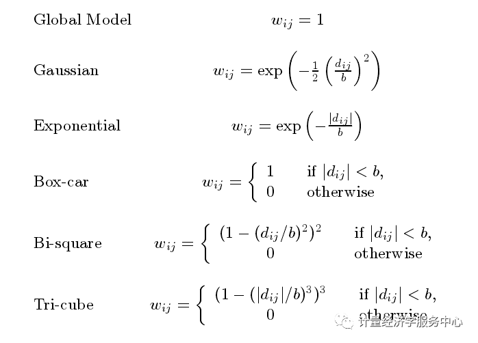
六个核函数的介绍:
Global Model(均值核函数)、Gaussian(高斯核函数)、Exponential、Box-car(盒状核函数)、Bi-square(二次核函数)、Tri-cude(立方体和函数)
2、spgwr函数
spgwr包需要安装,代码为:
install.packages("spgwr") library(spgwr)spgwr进行地理加权回归主要有两个非常重要的步骤,分别是带宽选择和回归。
带宽选择使用的是gwr.sel这个函数,语法格式为:
gwr.sel(formula, data=list(), coords, adapt=FALSE, gweight=gwr.Gauss, method = "cv", verbose = TRUE, longlat=NULL, RMSE=FALSE, weights, tol=.Machine$double.eps^0.25, show.error.messages = FALSE)选项含义为:
formula:regression model formula as in lm,表示R语言里面进行回归的方程式
data:model data frame as in lm, or may be a SpatialPointsDataFrame or SpatialPolygonsDataFrame object as defined in package sp 指定数据
coords: matrix of coordinates of points representing the spatial positions of the observations指定坐标(主要是经纬度,x对应经度,y对应纬度
gweight: 指定空间权重函数(代码中使用的gauss函数,以前默认的是gwr.bisquare()函数。
verbose:是否汇打印计算带宽的过程
method:指定带宽的计算方法
二、GW回归
GW 回归是探索因变量和自变量之间的空间变化关系,基本的GW回归是将通常的回归方法用于空间当中,最重要的是所有回归系数的估计都要加权,加权用到前面提到的核函数。
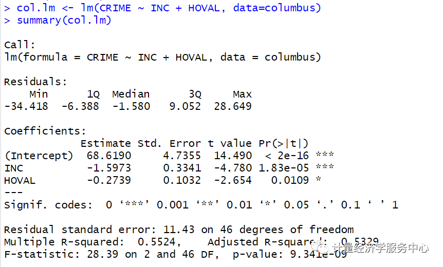
1、传统回归分析
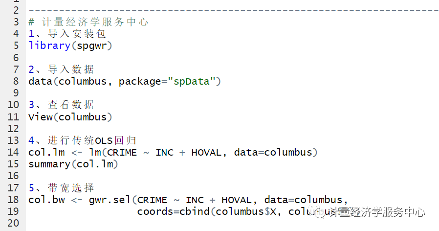
------------------------------------------------------------------------------------# 计量经济学服务中心1、导入安装包library(spgwr)2、导入数据data(columbus, package="spData")3、查看数据View(columbus)进行回归,代码为:
4、进行传统OLS回归col.lm <- lm(CRIME ~ INC + HOVAL, data=columbus)summary(col.lm)结果为:
2、带宽选择
------------------------------------------------------------------------------------# 计量经济学服务中心#5、带宽选择col.bw coords=cbind(columbus$X, columbus$Y))结果为:
> #5、带宽选择> col.bw + coords=cbind(columbus$X, columbus$Y))Bandwidth: 12.65221 CV score: 7432.209 Bandwidth: 20.45127 CV score: 7462.704 Bandwidth: 7.83213 CV score: 7323.545 Bandwidth: 4.853154 CV score: 7307.57 Bandwidth: 5.125504 CV score: 7322.796 Bandwidth: 3.012046 CV score: 6461.764 Bandwidth: 1.874179 CV score: 6473.378 Bandwidth: 2.475485 CV score: 6109.995 Bandwidth: 2.447721 CV score: 6098.372 Bandwidth: 2.228647 CV score: 6064.1 Bandwidth: 2.264538 CV score: 6060.774 Bandwidth: 2.280666 CV score: 6060.649 Bandwidth: 2.274969 CV score: 6060.601 Bandwidth: 2.2751 CV score: 6060.601 Bandwidth: 2.27506 CV score: 6060.601 Bandwidth: 2.275019 CV score: 6060.601 Bandwidth: 2.27506 CV score: 6060.601 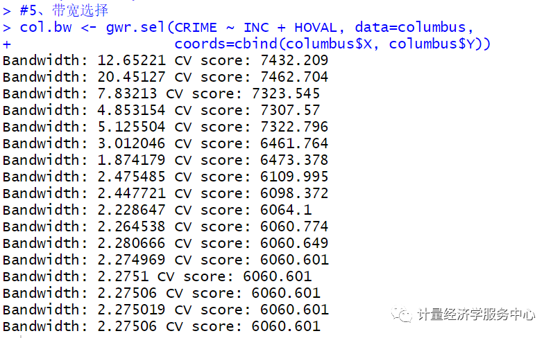
3、地理加权回归
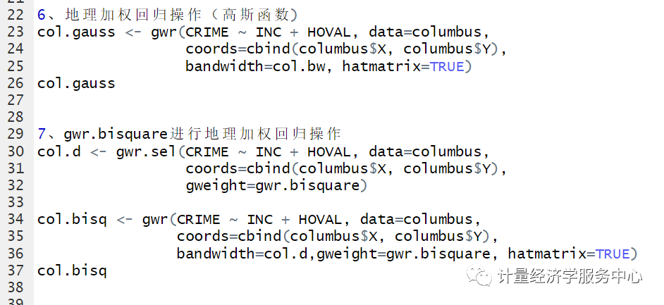
使用gwr进行地理加权回归,代码为:
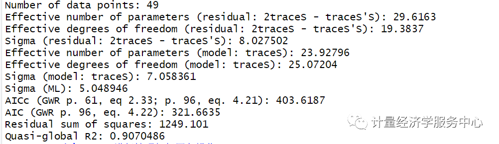
#6、地理加权回归操作(高斯函数)col.gauss <- gwr(CRIME ~ INC + HOVAL, data=columbus, coords=cbind(columbus$X, columbus$Y), bandwidth=col.bw, hatmatrix=TRUE)col.gauss结果为:
> #6、地理加权回归操作(高斯函数)> col.gauss + coords=cbind(columbus$X, columbus$Y),+ bandwidth=col.bw, hatmatrix=TRUE)> col.gaussCall:gwr(formula = CRIME ~ INC + HOVAL, data = columbus, coords = cbind(columbus$X, columbus$Y), bandwidth = col.bw, hatmatrix = TRUE)Kernel function: gwr.Gauss Fixed bandwidth: 2.27506 Summary of GWR coefficient estimates at data points: Min. 1st Qu. Median 3rd Qu. Max. GlobalX.Intercept. 23.233234 54.124872 63.902588 68.756460 80.900619 68.6190INC -3.130714 -1.912908 -0.984380 -0.368564 1.291075 -1.5973HOVAL -1.052811 -0.376735 -0.097394 0.030049 0.794577 -0.2739Number of data points: 49 Effective number of parameters (residual: 2traceS - traceS'S): 29.6163 Effective degrees of freedom (residual: 2traceS - traceS'S): 19.3837 Sigma (residual: 2traceS - traceS'S): 8.027502 Effective number of parameters (model: traceS): 23.92796 Effective degrees of freedom (model: traceS): 25.07204 Sigma (model: traceS): 7.058361 Sigma (ML): 5.048946 AICc (GWR p. 61, eq 2.33; p. 96, eq. 4.21): 403.6187 AIC (GWR p. 96, eq. 4.22): 321.6635 Residual sum of squares: 1249.101 Quasi-global R2: 0.9070486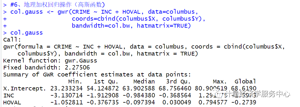
选择函数,代码和结果为:
> #7、gwr.bisquare进行地理加权回归操作> col.d + coords=cbind(columbus$X, columbus$Y), + gweight=gwr.bisquare)Bandwidth: 12.65221 CV score: 8180.619 Bandwidth: 20.45127 CV score: 7552.85 Bandwidth: 25.27136 CV score: 7508.227 Bandwidth: 23.68132 CV score: 7519.864 Bandwidth: 28.25033 CV score: 7491.85 Bandwidth: 30.09144 CV score: 7486.673 Bandwidth: 31.69353 CV score: 7483.663 Bandwidth: 31.08159 CV score: 7484.706 Bandwidth: 32.21945 CV score: 7482.846 Bandwidth: 32.54449 CV score: 7482.371 Bandwidth: 32.74538 CV score: 7482.088 Bandwidth: 32.86953 CV score: 7481.916 Bandwidth: 32.94626 CV score: 7481.812 Bandwidth: 32.99368 CV score: 7481.748 Bandwidth: 33.02299 CV score: 7481.708 Bandwidth: 33.04111 CV score: 7481.684 Bandwidth: 33.0523 CV score: 7481.669 Bandwidth: 33.05922 CV score: 7481.659 Bandwidth: 33.0635 CV score: 7481.654 Bandwidth: 33.06614 CV score: 7481.65 Bandwidth: 33.06777 CV score: 7481.648 Bandwidth: 33.06878 CV score: 7481.647 Bandwidth: 33.06941 CV score: 7481.646 Bandwidth: 33.06979 CV score: 7481.645 Bandwidth: 33.07003 CV score: 7481.645 Bandwidth: 33.07018 CV score: 7481.645 Bandwidth: 33.07027 CV score: 7481.645 Bandwidth: 33.07032 CV score: 7481.645 Bandwidth: 33.07037 CV score: 7481.645 Bandwidth: 33.07037 CV score: 7481.645 Warning message:In gwr.sel(CRIME ~ INC + HOVAL, data = columbus, coords = cbind(columbus$X, : Bandwidth converged to upper bound:33.0704149683672> > col.bisq + coords=cbind(columbus$X, columbus$Y),+ bandwidth=col.d,gweight=gwr.bisquare, hatmatrix=TRUE)> col.bisqCall:gwr(formula = CRIME ~ INC + HOVAL, data = columbus, coords = cbind(columbus$X, columbus$Y), bandwidth = col.d, gweight = gwr.bisquare, hatmatrix = TRUE)Kernel function: gwr.bisquare Fixed bandwidth: 33.07037 Summary of GWR coefficient estimates at data points: Min. 1st Qu. Median 3rd Qu. Max. GlobalX.Intercept. 68.30731 68.96074 69.26155 69.57103 71.64487 68.6190INC -1.72665 -1.64754 -1.61378 -1.56908 -1.46759 -1.5973HOVAL -0.33314 -0.30522 -0.28063 -0.25355 -0.18834 -0.2739Number of data points: 49 Effective number of parameters (residual: 2traceS - traceS'S): 4.604881 Effective degrees of freedom (residual: 2traceS - traceS'S): 44.39512 Sigma (residual: 2traceS - traceS'S): 11.3765 Effective number of parameters (model: traceS): 3.917653 Effective degrees of freedom (model: traceS): 45.08235 Sigma (model: traceS): 11.28946 Sigma (ML): 10.82875 AICc (GWR p. 61, eq 2.33; p. 96, eq. 4.21): 383.6983 AIC (GWR p. 96, eq. 4.22): 376.4297 Residual sum of squares: 5745.83 Quasi-global R2: 0.5724262◆◆◆◆
精彩回顾

点击上图查看:
《初级计量经济学及Stata应用:Stata从入门到进阶》

点击上图查看:
《零基础|轻松搞定空间计量:空间计量及GeoDa、Stata应用》

点击上图查看:
计量经济学小白必修课--网课《高级计量经济学及Eviews应用》震撼上架!

点击上图查看:
空间计量及Matlab应用课程