一、观测数据:
将观测数据整理成如下图所示
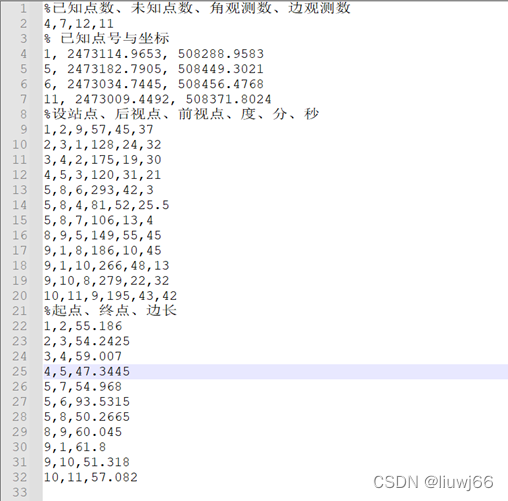
图 1 观测数据
为了给大家一个对数据的初步认识,将所得测量结果绘制到google earth上
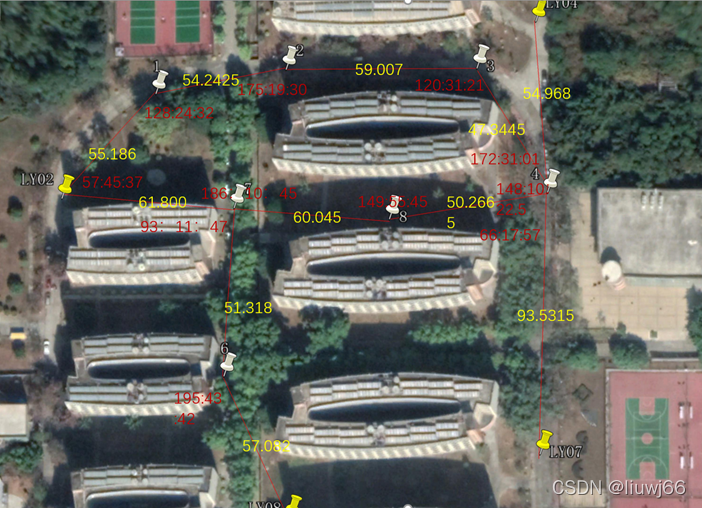
上图展示了本组测量的附和导线略图及观测数据、本次测量一种有11条边的观测数据、12个角的观测数据。在上图中的闭合环中,角度闭合差仅有4.5秒。初步说明了测量的可靠性。
三、程序结构:
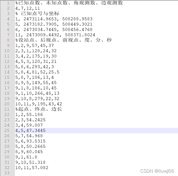
1. 读取观测数据
将观测数据整理成下图所示形式(注释仅为说明作用)、利用fgetl函数逐行读取并储存:
function [] = ReadObse(filename)
clc;
%********************read the observation data*************************
fid = fopen(filename);
%read the first line which includes
%number of control points, unknown points ,sides and angles
line1 = str2num(fgetl(fid));
num_known = line1(1);%known points
num_unknown = line1(2);%unknown points
num_angles = line1(3);%angles
num_sides = line1(4);%sides
%read the coordinates and indexs of known points:
for kkk = 1:num_known
        lines = str2num(fgetl(fid));
        idx_known(kkk) = lines(1);%index
        x_known(kkk) = lines(2);%x
        y_known(kkk) = lines(3);%y
end
%read the obeservation angles and station index
for ttt  =1: num_angles
        liness  =str2num(fgetl(fid));
        sta_now(ttt) = liness(1);%present station
        sta_after(ttt) = liness(2);%backward station
        sta_before(ttt) = liness(3);%front station
        angles(ttt) = liness(4)+liness(5)/60+ liness(6)/3600;%observation angles
end
%read the observation sides and station index
for tst = 1:num_sides
        lined = str2num(fgetl(fid));
        pts_start(tst) = lined(1);%read index of start points
        pts_end(tst) = lined(2);%read index of end points
        sides(tst) = lined(3);%read the observation sides
end
end
2.利用有向图存储边长观测数据,利用数组存储角数据
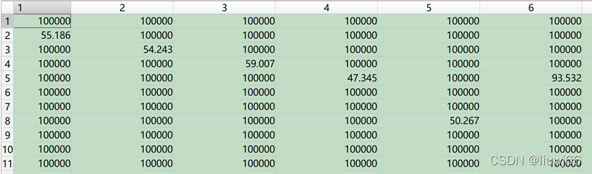
%build a side network
num_total = num_unknown + num_known;
side_net  =100000*ones(num_total,num_total);

for tks = 1:num_sides
        starts = pts_start(tks);
        ends = pts_end(tks);
        side_net(starts, ends) = sides(tks);
end
3. 迭代计算初始坐标:利用Dijkstra最短路径算法
假定初始方位角为0,利用Dijkstra算法求出某一控制点到另一控制点的最短路径。沿该路径迭代计算初始方位角及初始坐标,直到方位角的改正值满足一定阈值。遍历所有从某一控制点到另一控制点的路径(若有4个控制点,则有16条路径),最后将所求取的所有点的坐标进行平均作为平差的初值。
计算初始值 主函数:
function [x0, y0] = CalInitial(pts_first,pts_last)
        x01 =[];y01 = [];
        x0 = NaN(1,12);
        y0 = NaN(1,12);
        load('Observation.mat')
        idx_start = idx_known(pts_first);
        idx_end = idx_known(pts_last);
        [dist,path_initial] = DIJK(side_net, idx_start, idx_end);
        %set the initial azimuth angle in degree
         lth_path = length(path_initial);
         if(lth_path > 2)
                x01(1) = x_known((find(idx_known == idx_start)));
                y01(1) = y_known((find(idx_known == idx_start)));
                al_hypo = 1;%hypothsised azimuth angle
                al_real = 0;
                al_path(1) = 0;% al_path store the azimuth angle along the path
                %calculate the initial coordinate through the path_origin
                while(abs(al_hypo - al_real) >= 0.5)
                        delta_al = - al_hypo + al_real;
                        al_path(1) = al_path(1)+delta_al;
                        lth_path = length(path_initial);
                         for ts  = 2:lth_path-1
                                idx1 = find(sta_now == path_initial(ts));
                                idx2 = find(sta_before == path_initial(ts+1));
                                idx3 = find(sta_after == path_initial(ts-1));
                                idx12 = intersect(idx1, idx2);
                                idx = intersect(idx12, idx3);
                                if length(idx) > 0
                                al_path(ts) = al_path(ts-1) - 180 + angles(idx);
                                else return
                                end
                        end

                        for ts = 2:lth_path
                                x01(ts) = x01(ts-1) + side_net(path_initial(ts-1),path_initial(ts))*cosd(al_path(ts-1));
                                y01(ts) = y01(ts-1) + side_net(path_initial(ts-1),path_initial(ts))*sind(al_path(ts-1));
                        end

                        al_hypo =  atan2d((y01(lth_path) - y01(1)),(x01(lth_path) - x01(1)));
                        al_real =  atan2d((y_known(find(idx_known == idx_end)) - y01(1)),((x_known(find(idx_known == idx_end)) - x01(1))));
                        delta_al = - al_hypo + al_real;
                end
                x0(path_initial) = x01;
                y0(path_initial) = y01;
         end
end
Dijkstra算法构建求取路径
function [distance,path] = DIJK(W, st, e)
%DIJK Summary of this function goes here
%   W  权值矩阵   st 搜索的起点   e 搜索的终点
n=length(W);%节点数
D = W(st,:);
visit= ones(1:n); visit(st)=0;
parent = zeros(1,n);%记录每个节点的上一个节点

path =[];

for i=1:n-1
    temp = [];
    %从起点出发,找最短距离的下一个点,每次不会重复原来的轨迹,设置visit判断节点是否访问
    for j=1:n
       if visit(j)
           temp =[temp D(j)];
       else
           temp =[temp inf];
       end

    end

    [value,index] = min(temp);

    visit(index) = 0;

    %更新 如果经过index节点,从起点到每个节点的路径长度更小,则更新,记录前趋节点,方便后面回溯循迹
    for k=1:n
        if D(k)>D(index)+W(index,k)
           D(k) = D(index)+W(index,k);
           parent(k) = index;
        end
    end


end

distance = D(e);%最短距离
%回溯法  从尾部往前寻找搜索路径
t = e;
while t~=st && t>0
 path =[t,path];
  p=parent(t);t=p;
end
path =[st,path];%最短路径
end
4. 将求取的所有点的坐标进行平差。
在列边长的观测方程时分以下几种情况讨论:
1)起点为控制点、终点为未知点
2)起点为未知点、终点为控制点
3)起点、终点均为未知点
在列角度的观测方程时分以下几种情况讨论:
1)设站点为控制点、前视、后视均为未知点
2)设站点为控制点、前视、后视有一个未知点
3)设站点为未知点、前视、后视有一个控制点
4)设站点为未知点、前视、后视无控制点
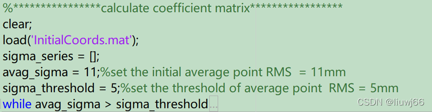
while avag_sigma > sigma_threshold
        vs = [];
        ls = [];
        con_index = idx_known;
        idx_all = 1:(num_unknown+num_known);
        other_index = setdiff(idx_all,idx_known);
        sp0 = pts_start; ep0 = pts_end;
        lth0 = sides;
        %calculation the V = B*x - l by observations of sides
        for ikk = 1:num_sides
                vs(ikk, :) = zeros(2*num_unknown,1);
                sps = sp0(ikk);eps = ep0(ikk);
                if_con1  = sum((con_index == sps));
                if_con2  =sum(con_index == eps);
                ls(ikk) = lth0(ikk) - sqrt((x0(eps) - x0(sps)).^2+(y0(eps) - y0(sps)).^2);
                v1 = (x0(eps) - x0(sps))/lth0(ikk);
                v2 = (y0(eps) - y0(sps))/lth0(ikk);
                %consider three types of equation
                if (if_con1 == 1)&& (if_con2 == 0)
                      num = find(other_index == eps);
                      vs(ikk, 2*num) = v2; vs(ikk, 2*num-1) = v1;
               elseif (if_con1 == 0)&& (if_con2 == 1)
                        num = find(other_index == sps);
                        vs(ikk, 2*num) = -v2; vs(ikk, 2*num-1) = -v1;
                elseif (if_con1 == 0)&& (if_con2 == 0)
                        num1 = find(other_index == sps);
                        num2 = find(other_index == eps);
                        vs(ikk, 2*num2) = v2; vs(ikk, 2*num2-1) = v1;
                        vs(ikk, 2*num1) = -v2; vs(ikk, 2*num1-1) = -v1;
                end
        end
        ls = ls'*1000;
        deg0 = angles;
        sta_f0 = sta_before;
        sta_b0 = sta_after;
        sta_n0 = sta_now;
        rou = 180*60*60/pi;
        va = [];
        la = [];
       %calculation the V = B*x - l by observations of angles
        for akk = 1:num_angles
               fp = sta_f0(akk); ap = sta_b0(akk); np = sta_n0(akk);
               va(akk, :) = zeros(2*num_unknown, 1);
                if_conn  = sum((con_index == np));
                if_conf = sum(con_index == fp);
                if_cona = sum(con_index == ap);
                d1 = atan2d((y0(ap) - y0(np)), (x0(ap) - x0(np)));
               d2 = atan2d((y0(fp) - y0(np)), (x0(fp) - x0(np)));
                d1k(akk) = d1;
                d2k(akk) = d2;
                degd = d2 - d1;
                if degd<0
                         degd = degd + 360;
                end
               deltad(akk) = degd;
               la(akk) = deg0(akk)  - degd;
               dist_a(akk)  = side_net(ap,np);
               if dist_a(akk) > 1000
                       dist_a(akk) = side_net(np,ap);
               end
               dist_f(akk)  = side_net(np,fp);
               if dist_f(akk) > 1000
                       dist_f(akk) = side_net(fp,np);
               end
                numf = find(other_index == fp);
                numa = find(other_index == ap);
                numn = find(other_index == np);
               vax = (x0(ap) - x0(np))/dist_a(akk)^2;
               vay = (y0(ap) - y0(np))/dist_a(akk)^2;
               vfx = (x0(fp) - x0(np))/dist_f(akk)^2;
               vfy = (y0(fp) - y0(np))/dist_f(akk)^2;
               %consider 5 types of equation
                if(if_conn == 1)&&(if_cona == 0)&&(if_conf == 0)
                       va(akk, 2*numf) = -vfx;
                       va(akk, 2*numf-1) = vfy;
                       va(akk, 2*numa) = vax;
                       va(akk, 2*numa-1) = -vay;
                elseif(if_conn == 0)&&(if_cona == 0)&&(if_conf == 0)
                       va(akk, 2*numf) = -vfx;
                       va(akk, 2*numf-1) = vfy;
                       va(akk, 2*numa) = vax;
                       va(akk, 2*numa-1) = -vay;
                       va(akk, 2*numn) = vfx - vax;
                       va(akk, 2*numn-1) = vay  -  vfy;
                       elseif(if_conn == 0)&&(if_cona == 0)&&(if_conf == 1)
                       va(akk, 2*numa) = vax;
                       va(akk, 2*numa-1) = -vay;
                       va(akk, 2*numn) = vfx - vax;
                       va(akk, 2*numn-1) = vay  -  vfy;
                      elseif(if_conn == 0)&&(if_cona == 1)&&(if_conf == 1)
                       va(akk, 2*numn) = vfx - vax;
                       va(akk, 2*numn-1) = vay  -  vfy;
                     elseif(if_conn == 0)&&(if_cona == 1)&&(if_conf == 0)
                       va(akk, 2*numf) = -vfx;
                       va(akk, 2*numf-1) = vfy;
                       va(akk, 2*numn) = vfx - vax;
                       va(akk, 2*numn-1) = vay  -  vfy;
                end
        end
         va = rou*va/1000;
         la = la*3600;
         la = la';
        %set the weight matrix P
        os = 2 + 2*10^(-6)*lth0*10^3;
        oa = 2*ones(1,num_angles);
        o = [os oa];
        p = diag([4./o.^2]);
        %V = B*x - l; Nbb*x = w;
        B = [vs; -va];
        l = [ls; la];
        nbb = B'*p*B;
        w = B'*p*l;
        x = inv(nbb)*w;
        xs = x0(other_index) + x(1:2:2*num_unknown)'/1000;
        ys = y0(other_index) + x(2:2:2*num_unknown)'/1000;
        v= B*x -l;
        sigma0 = sqrt(v'*p*v/8);
        sigma_all = sigma0*sqrt(inv(nbb));
        a = diag(sigma_all);
        sigma_xy = sqrt(a(1:2:2*num_unknown).^2+a(2:2:2*num_unknown).^2);
        avag_sigma = mean(sigma_xy);
        sigma_series = [sigma_series mean(sigma_xy)];
        xs_adjust(con_index) = x0(con_index);
        ys_adjust(con_index) = y0(con_index);
        xs_adjust(other_index) = xs;
        ys_adjust(other_index) = ys;
        x0 = xs_adjust; y0 = ys_adjust;
%         x0(idx_known) = x_known;
%          y0(idx_known) = y_known;
end
5. 迭代平差直到满足平均点位中误差的阈值或收敛。
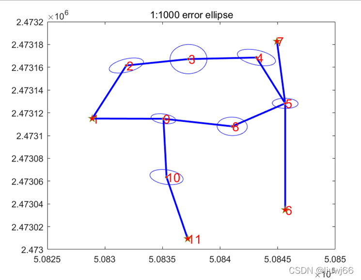
6. 可视化:
%plot the first 100 average RMS series of the iterations
%plot(sigma_series(1),'-s','linewidth',1.5);
set(gcf,'color','white')
xlabel('times of iteration');
ylabel('average MSE of points(mm) ')
%plot the traverse net and error ellipse
num_all  = num_known+num_unknown;
for ts = 1:num_all
        st = pts_start(ts);
        en = pts_end(ts);
        plot([ys_adjust(st),ys_adjust(en)],[xs_adjust(st),xs_adjust(en)],'linewidth',2,'color','blue');
        hold on;
        text(ys_adjust(ts),xs_adjust(ts),num2str(ts),'Color','red','FontSize',14)
end
scatter(ys_adjust(con_index),xs_adjust(con_index),80,'Marker','p','MarkerFaceColor','red');
scatter(ys_adjust(other_index),xs_adjust(other_index),10,'Marker','o','MarkerFaceColor','red');
Qxx = inv(nbb);
for tst = 1:2:2*num_unknown
        qxx = Qxx(tst,tst); qyy = Qxx(tst+1,tst+1);
        qxy = Qxx(tst,tst+1);
        K((tst+1)/2) = sqrt((qxx-qyy)^2 + 4*qxy^2);
        qee = (qxx+qyy+K((tst+1)/2));
        qff = (qxx+qyy- K((tst+1)/2));
        E((tst+1)/2) = sigma0*sqrt(qee)/1;
        F((tst+1)/2) = sigma0*sqrt(qff)/1;
        phie((tst+1)/2) = atan2(qee-qff,qxy);

end
for yy = 1:num_unknown
        idxx = other_index(yy);
                circle = 0:0.01:2*pi;
                xout = xs_adjust(idxx) + 2*E(yy)*cos(phie(yy))*cos(circle) - 2*F(yy)*sin(phie(yy))*sin(circle);
                yout = ys_adjust(idxx) + 2*E(yy)*sin(phie(yy))*cos(circle) + 2*F(yy)*cos(phie(yy))*sin(circle);
                plot(yout,xout,'-b');
                hold on;
end
set(gcf,'color','white');
title('1:1000 error ellipse');版权声明:本文为go_with_the_wind原创文章,遵循CC 4.0 BY-SA版权协议,转载请附上原文出处链接和本声明。