Python qutip用法(举例介绍)
一、N原子系综自旋概率分布
from qutip import spin_coherent,jmat,spin_q_function,plot_spin_distribution_3d,mesolve
import numpy as np
import matplotlib.pyplot as plt

n=30#原子数
j = n//2
psi0 = spin_coherent(j, np.pi/2, 0)#设置初态,自旋相干态
Jz=jmat(j,"z")
H=Jz**2#系统的哈密顿量

tlist=np.linspace(0,1,100)#时间列表
result=mesolve(H,psi0,tlist)#态随时间的演化

theta=np.linspace(0, np.pi, 100)
phi=np.linspace(0, 2*np.pi, 100)
Q1, THETA1, PHI1 = spin_q_function(result.states[0], theta, phi)
Q2, THETA2, PHI2 = spin_q_function(result.states[30], theta, phi)
Q3, THETA3, PHI3 = spin_q_function(result.states[60], theta, phi)
Q4, THETA4, PHI4 = spin_q_function(result.states[90], theta, phi)

fig = plt.figure(figsize=(8,8))
ax1 = fig.add_subplot(221,projection='3d')
ax2 = fig.add_subplot(222,projection='3d')
ax3 = fig.add_subplot(223,projection='3d')
ax4 = fig.add_subplot(224,projection='3d')

plot_spin_distribution_3d(Q1, THETA1, PHI1,fig=fig,ax=ax1)
plot_spin_distribution_3d(Q2, THETA2, PHI2,fig=fig,ax=ax2)
plot_spin_distribution_3d(Q3, THETA3, PHI3,fig=fig,ax=ax3)
plot_spin_distribution_3d(Q4, THETA4, PHI4,fig=fig,ax=ax4)

for ax in [ax1,ax2,ax3,ax4]:
    ax.view_init(0.5*np.pi, 0)
    ax.axis('off')#不显示坐标轴
#fig.savefig("1.png",dpi=400)
plt.show()
运行结果:
二、原子与光场相互作用
from qutip import jmat,mesolve,fock,spin_state,expect,tensor,qeye,destroy
import numpy as np
import matplotlib.pyplot as plt
from matplotlib import rcParams

config = {
    "font.family":'serif',
    "font.size": 15,
    "mathtext.fontset":'cm',
    "font.serif": ['Arial'],
}

rcParams.update(config)

j = 1/2
Jp=jmat(j,'+')#原子的升算符
J_=jmat(j,'-')#原子的降算符
Jx=jmat(j,'x')#原子的Jx算符
Jy=jmat(j,'y')#原子的Jy算符,这里的j是虚数单位
Jz=jmat(j,'z')#原子的Jz算符

a=destroy(50)#光场的湮灭算符,50是矩阵的维度。理论上维度应该是无限大,但实际计算只能给定足够大的有限维度
a_plus=a.dag()#光场的产生算符
eye=qeye(50)#单位阵
psi0 = tensor(fock(50,0),spin_state(j,0))#设置系统的初态为直积态 |0>×|↑>

H=tensor(a,Jp)+tensor(a_plus,J_)#系统的哈密顿量
tlist=np.linspace(0,10,1000)#时间列表
result=mesolve(H,psi0,tlist)#态随时间的演化

fig=plt.figure(figsize=(8,6))

(ax1,ax2),(ax3,ax4) = fig.subplots(2,2)
ax1.plot(tlist,expect(tensor(eye,Jx),result.states),color='blue');ax1.set_ylabel(r"$\langle \hat{J}_x \rangle$")#Jx的平均值随时间变化图
ax2.plot(tlist,expect(tensor(eye,Jz),result.states),color='blue');ax2.set_ylabel(r"$\langle \hat{J}_z \rangle$")#Jz的平均值随时间变化图
ax3.plot(tlist,expect(tensor(a_plus*a,qeye(2)),result.states),color='blue');ax3.set_ylabel(r"$\langle \hat{a}^{\dag} a \rangle$")#光子数的平均值随时间变化图
ax4.plot(tlist,expect(tensor(eye,Jx**2+Jy**2+Jz**2),result.states),color='blue');ax4.set_ylabel(r"$\langle \hat{J}^2 \rangle$")#J平方的平均值随时间变化图

for ax in fig.axes:
    ax.tick_params(direction="in",axis='both',labelsize=15,length=4,width=1.2)
    ax.set_xlim(0,tlist[-1])
    [spine.set_linewidth(1.2) for spine in ax.spines.values()]
    ax.set_xlabel(r"$t$",size=20)
ax1.set_ylim(-1.1,1.1)
ax4.set_ylim(0,2.2)
fig.tight_layout()
#fig.subplots_adjust(top=None,bottom=None,left=None,right=None,wspace=0.4,hspace=0.4)
fig.show()
运行结果: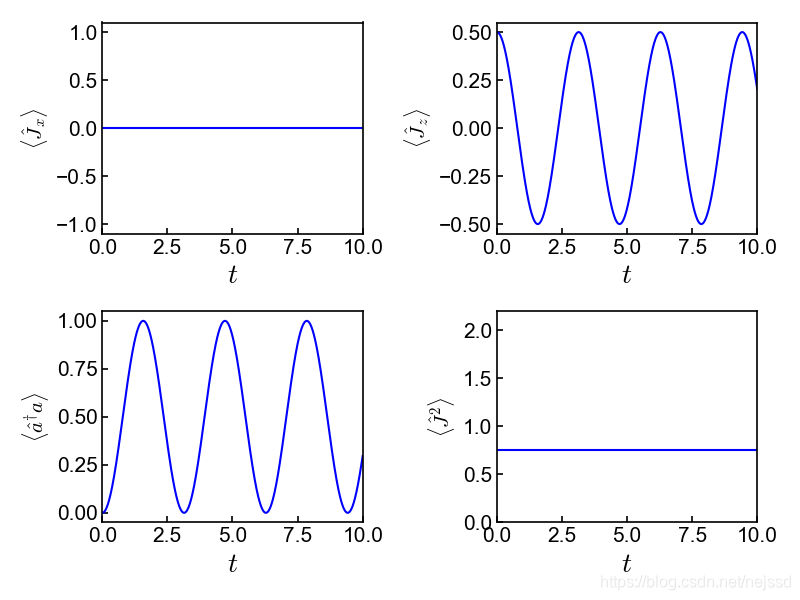
版权声明:本文为nejssd原创文章,遵循CC 4.0 BY-SA版权协议,转载请附上原文出处链接和本声明。