As I had promised in my previous article, now, it’s time to complete our discussion on evaluation metrics for classification problems. Today, we are going to discuss the limitation of the AUC-ROC technique.

正如我在上一篇文章中所承诺的那样，现在是时候完成关于分类问题评估指标的讨论了。 今天，我们将讨论AUC-ROC技术的局限性 。

First of all, before the limitation, it’s important to understand, how the ROC Curve forms.

首先，在限制之前，了解ROC曲线的形成方式非常重要。

So, firstly, we will begin with a thorough discussion on how ROC Curve forms and then, we will discuss its limitation, as the explanation of the limitation comes from the theory of the formation of ROC Curve.

因此，首先，我们将详细讨论ROC曲线的形成方式，然后再讨论其局限性，因为对局限性的解释来自于ROC曲线的形成理论。

介绍 (Introduction)

So, before moving to the ROC, it’s very important to discuss the True Positive Rate (T.P.R)& False Positive Rate (F.P.R).

因此，在转向中华民国之前，讨论真正利率(TPR)和假正利率(FPR)非常重要。

The mathematical formula of T.P.R is given below:

TPR的数学公式如下：

& the mathematical formula of F.P.R is given below:

FPR的数学公式如下：

Now, without wasting time, let’s jump onto the AUR-ROC technique.

现在，在不浪费时间的情况下，让我们开始使用AUR-ROC技术。

AUC-ROC曲线 (AUC-ROC Curve)

A.U.C means Area under the curve which we calculate of the ROC (Receiver Operations Characteristics) curve.

AUC是指我们计算的ROC(接收机工作特性)曲线的曲线下面积。

AUC-ROC technique basically gives us a tradeoff between True Positive Rate (T.P.R) & False Positive Rate (F.P.R).

AUC-ROC技术基本上使我们在真正率(TPR)和假正率(FPR)之间进行权衡。

Originally, ROC Curve was used for distinguishing ‘noise’ from ‘not noise’.

最初，ROC曲线用于区分“噪声”与“非噪声”。

Now coming to the formation of the ROC Curve.

现在开始形成ROC曲线 。

Now, let’s begin with the threshold principle to understand the formation of the ROC Curve.

现在，让我们从阈值原理开始，了解ROC曲线的形成。

门槛原则 (Threshold Principle)

The threshold principle is used to calculate the True Positive Rate & False Positive Rate.

阈值原理用于计算正确率和错误率。

Let’s take an example.

让我们举个例子。

Suppose we have the following table of Actual values & Predicted values.

假设我们有下表“实际值”和“预测值”。

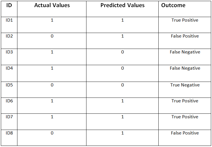
Now, it’s important to understand that any Machine learning algorithm, actually gives the probability of any outcome.

现在，重要的是要了解任何机器学习算法实际上都会给出任何结果的可能性 。

The function that you apply, internally applies a threshold on the probability to decide a particular outcome.

您应用的函数会在内部应用阈值来确定特定结果。

In the above table, the predicted values are those, which you get as the output from a Machine learning algorithm. Now, let’s see a new table below.

在上表中， 预测值是您从机器学习算法的输出中获得的值。 现在，让我们在下面看到一个新表。

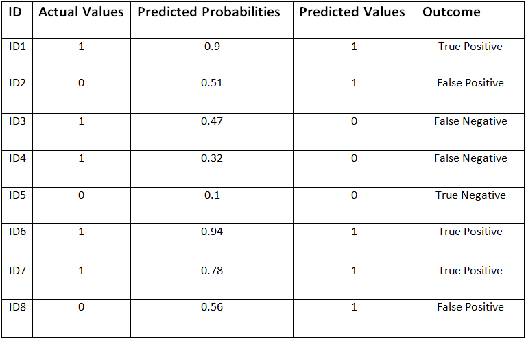
Here, the probabilities are for getting one (1) as the output.

在这里，概率是用于获得一(1)作为输出。

Predicting probabilities is the work that is actually expected by an ML algorithm to do, rest is just applying a threshold.

预测概率是ML算法实际上要完成的工作，其余只是应用阈值。

In the above table, the “Predicted Values” are the result of applying the threshold on the “Predicted Probabilities”. For example, in the above table, threshold = 0.5, which means that if “Predicted Probabilities” is greater than or equal to 0.5, the predicted value will be 1, else 0.

在上表中，“预测值”是在“预测概率”上应用阈值的结果。 例如，在上表中，阈值= 0.5，这意味着如果“预测概率”大于或等于0.5，则预测值将为1，否则为0。

Now, a common question that may come in mind is that, what if I increase the threshold. Well, Increasing/Decreasing threshold will effect True Positives, False Positives, True Negatives, and False Negatives. & that’s what we going to do in the next few minutes. We are going to play with the thresholds.

现在，可能会想到的一个常见问题是，如果我提高阈值会怎样？ 好吧，增加/减少阈值将影响“真阳性”，“假阳性”，“真阴性”和“假阴性”。 这就是我们接下来几分钟要做的事情。 我们将使用阈值。

Now we have got enough knowledge about the thresholds & it’s workings, let’s move on to the working & formation of the ROC curve

现在我们对阈值及其工作原理有了足够的了解，让我们继续研究ROC曲线的工作和形成

ROC曲线的形成 (Formation of R.O.C Curve)

There are a few steps required for the formation of the R.O.C curve. For better understanding, at each step, we will solve an example which we will take in the beginning.

形成ROC曲线需要几个步骤。 为了更好地理解，在每一步中，我们将解决一个示例，我们将从一开始就采用该示例。

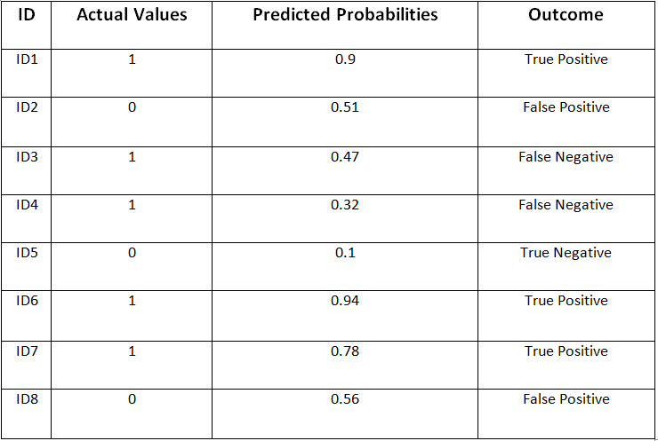
So, let’s take the same table as an example, which we took above. But, since our objective is to find the ROC Curve, we will not take “Predicted values” into account.

因此，让我们以上面的表格为例。 但是，由于我们的目标是找到ROC曲线，因此我们将不考虑“预测值”。

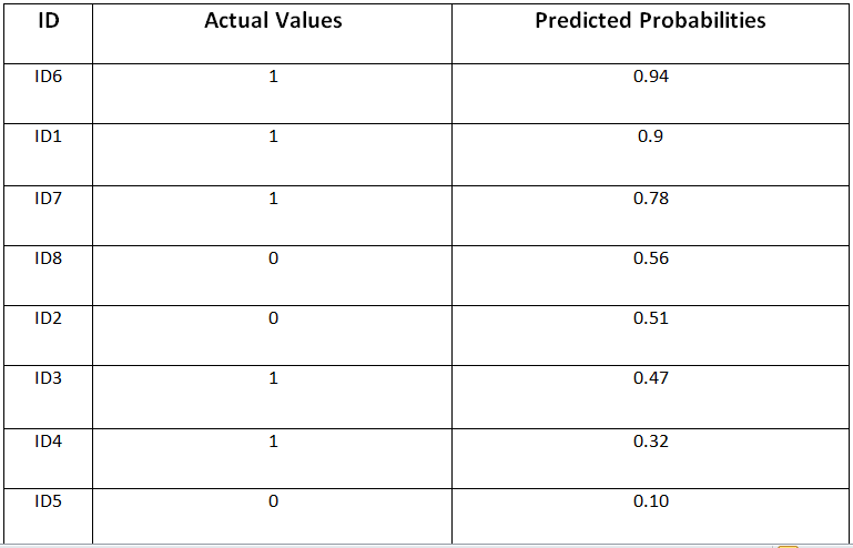
Step 1: Arrange all the rows according to decreasing order

步骤1：按照降序排列所有行

Now, we have to arrange all the rows in the descending order according to the predicted probabilities. Here’s what we get.

现在，我们必须根据预测的概率按降序排列所有行。 这就是我们得到的。

Step 2: Take the first probability as the threshold.

步骤2：以第一个概率为阈值。

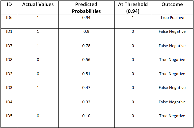
Step 3: T.P.R (True Positive Rate) and F.P.R (False Positive Rate)

步骤3：TPR(正确率)和FPR(错误率)

Now, by the T.P.R & F.P.R formula, we got,

现在，根据TPR和FPR公式，

True Positive Rate = 1/5 = 0.2

真实正利率= 1/5 = 0.2

False Positive Rate = 0

误报率= 0

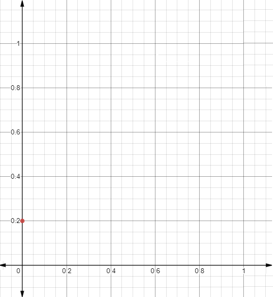
Now, we are going to plot our first point on the ROC curve. The F.P.R is on the x-axis & T.P.R is on the y-axis.

现在，我们将在ROC曲线上绘制第一个点。 FPR在x轴上，TPR在y轴上。

The following graph is obtained:

获得下图：

Step 4: Repeat steps 2 & 3 & take the next probability as threshold till end

步骤4：重复步骤2和3，并以下一个概率为阈值，直到结束

Now, it’s time to go to step 2 & instead we will take threshold = 0.9.

现在，该进行第2步了，取而代之的是，我们将阈值= 0.9。

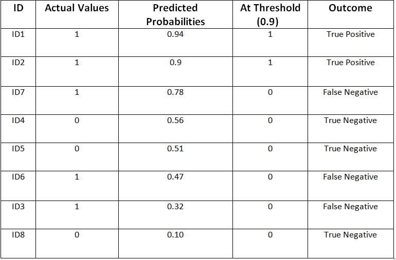
Step 3:

第三步：

Now, again we have to calculate T.P.R & F.P.R.

现在，我们必须再次计算TPR和FPR

Step 4: T.P.R (True Positive Rate) and F.P.R (False Positive Rate)

步骤4：TPR(正确率)和FPR(错误率)

Now, by the T.P.R & F.P.R formula, we got,

现在，根据TPR和FPR公式，

True Positive Rate = 2/5 = 0.4

真实肯定率= 2/5 = 0.4

False Positive Rate = 0

误报率= 0

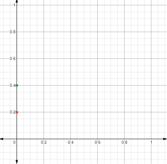
Now, we are going to plot our 2nd point on the ROC curve. The F.P.R is on the x-axis & T.P.R is on the y-axis.

现在，我们将在ROC曲线上绘制第二点。 FPR在x轴上，TPR在y轴上。

The updated Graph is shown below.

更新后的图表如下所示。

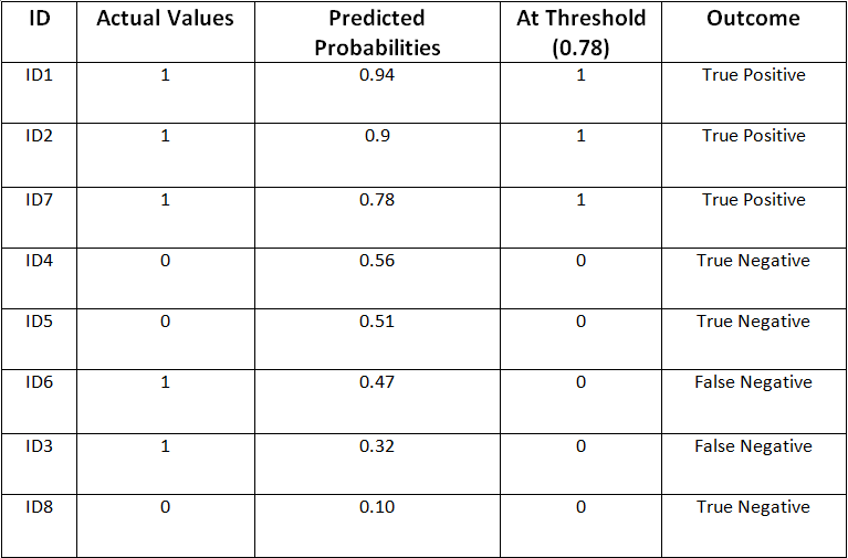
Now, according to step 4, we have to repeat step 2 with threshold = 0.78. Below is the table we got.

现在，根据步骤4，我们必须以阈值= 0.78重复步骤2。 下面是我们得到的表。

Again Calculation of T.P.R & F.P.R

再次计算TPR和FPR

True Positive Rate = 3/5 = 0.6

真实正利率= 3/5 = 0.6

False Positive Rate = 0

误报率= 0

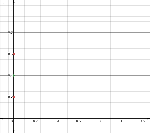
Now, we are going to plot our 3rd point on the ROC curve. The F.P.R is on the x-axis & T.P.R is on the y-axis.

现在，我们将在ROC曲线上绘制第三个点。 FPR在x轴上，TPR在y轴上。

The updated Graph is shown below.

更新后的图表如下所示。

….. (Repeating the process until we reach the last, taking the last probability as the threshold)

…..(以最后的概率为阈值，重复此过程直到达到最后一个)

Now, if we repeat the process until we reach the end, we will get the following graph.

现在，如果我们重复该过程直到结束，我们将得到以下图形。

(Here, I’m skipping the steps just for the sake of the length of this article.)

(在这里，仅为了本文的篇幅，我跳过了这些步骤。)

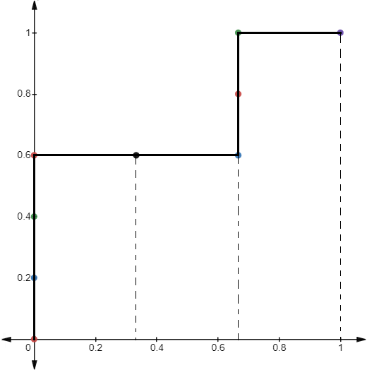
The above graph may seem like a strange one, but, I’ve taken a casual data with only 8 rows. But, when you’re dealing with real-world problems, you’ll most probably get a standard 2D curve, just like what a standard ROC curve looks like.I think it’s quite clear now.

上面的图似乎是一个奇怪的图，但是，我仅使用了8行的临时数据。 但是，当您处理现实世界中的问题时，您很可能会获得标准2D曲线，就像标准ROC曲线的样子一样。我认为现在已经很清楚了。

Now, I think you have understood the formation of the ROC Curve. The AUC is just to check the accuracy. The AUC of the above graph is = 0.736, which means that our model is better than the random one.

现在，我认为您已经了解了ROC曲线的形成。 AUC只是为了检查准确性。 上图的AUC = 0.736，这意味着我们的模型优于随机模型。

Now, since you’ve understood the formation of the ROC Curve, it’s time to discuss the limitation, which is the ultimate objective of this article.

现在，由于您已经了解了ROC曲线的形成，是时候讨论该限制了，这是本文的最终目标。

AUC-ROC技术的局限性 (Limitation of the AUC-ROC Technique)

The limitation of the AUC-ROC technique is that we can’t compare 2 different models with this.

AUC-ROC技术的局限性是我们不能与此比较两个不同的模型。

Since you’ve already understood, how the ROC curve forms, you may notice that the ROC Curve formed is basically dependent on the order of the probability.

既然您已经了解了ROC曲线的形成方式，那么您可能会注意到所形成的ROC曲线基本上取决于概率的顺序。

We have already discussed above that the main objective of any Machine Learning model is to find the probability, if we change the Machine Learning model, the probabilities will change, but the area of the ROC curve depends upon the order, not the probability itself. So, if we change the Machine Learning model, the order will remain unchanged, condition applied that no predicted probability will remain the same.

上面我们已经讨论了任何机器学习模型的主要目标是找到概率，如果我们更改机器学习模型，则概率将改变，但是ROC曲线的面积取决于顺序 ，而不是概率本身。 因此，如果我们更改机器学习模型，则顺序将保持不变，并且条件是没有预测的概率将保持不变。

Therefore, we can’t compare 2 Machine Learning models with the AUC-ROC technique.

因此，我们无法将两种机器学习模型与AUC-ROC技术进行比较 。

So, this is the reason for the limitation of the AUC-ROC curve. I hope, I’ve explained it properly. So, with this, we can complete our discussion on the evaluation metrics for classification problems.

因此，这就是限制AUC-ROC曲线的原因。 希望我已经正确解释了。 因此，这样就可以完成对分类问题评估指标的讨论。

In this article, we have discussed the reason for the limitation of the AUC-ROC technique. But, before going to evaluation metrics, there are several important topics or steps like model training, data exploration, Feature Engineering, Data Analysis, etc. In the future, I will post more articles on these topics. Till then, stay tuned.

在本文中，我们讨论了限制AUC-ROC技术的原因。 但是，在评估指标之前，有几个重要的主题或步骤，例如模型训练，数据探索，特征工程，数据分析等。将来，我将针对这些主题发布更多文章。 直到那时，请继续关注。