EM for PCA
With complete information
- If we knew z zz for each x xx, estimating A AA and D DD would be simple
x = A z + E x=A z+Ex=Az+E
P ( x ∣ z ) = N ( A z , D ) P(x \mid z)=N(A z, D)P(x∣z)=N(Az,D)
- Given complete information ( x 1 , z 1 ) , ( x 2 , z 2 ) \left(x_{1}, z_{1}\right),\left(x_{2}, z_{2}\right)(x1,z1),(x2,z2)
argmax A , D ∑ ( x , z ) log P ( x , z ) = argmax A , D ∑ ( x , z ) log P ( x ∣ z ) \underset{A, D}{\operatorname{argmax}} \sum_{(x, z)} \log P(x, z)=\underset{A, D}{\operatorname{argmax}} \sum_{(x, z)} \log P(x \mid z)A,Dargmax(x,z)∑logP(x,z)=A,Dargmax(x,z)∑logP(x∣z)
= argmax A , D ∑ ( x , Z ) log 1 ( 2 π ) d ∣ D ∣ exp ( − 0.5 ( x − A z ) T D − 1 ( x − A z ) ) =\underset{A, D}{\operatorname{argmax}} \sum_{(x, Z)} \log \frac{1}{\sqrt{(2 \pi)^{d}|D|}} \exp \left(-0.5(x-A z)^{T} D^{-1}(x-A z)\right)=A,Dargmax(x,Z)∑log(2π)d∣D∣1exp(−0.5(x−Az)TD−1(x−Az))
- We can get a close form solution: A = X Z + A = XZ^{+}A=XZ+
- But we don’t have Z ZZ => missing
With incomplete information
- Initialize the plane
- Complete the data by computing the appropriate z zz for the plane
- P ( z ∣ X ; A ) P(z|X;A)P(z∣X;A) is a delta, because E EE is orthogonal to A AA
- Reestimate the plane using the z zz
- Iterate
Linear Gaussian Model
- PCA assumes the noise is always orthogonal to the data
- Not always true
- The noise added to the output of the encoder can lie in any direction (uncorrelated)
- We want a generative model: to generate any point
- Take a Gaussian step on the hyperplane
- Add full-rank Gaussian uncorrelated noise that is independent of the position on the hyperplane
- Uncorrelated: diagonal covariance matrix
- Direction of noise is unconstrained
With complete information
x = A z + e x=A z+ex=Az+e
P ( x ∣ z ) = N ( A z , D ) P(x \mid z)=N(A z, D)P(x∣z)=N(Az,D)
- Given complete information X = [ x 1 , x 2 , … ] , Z = [ z 1 , z 2 , … ] X=\left[x_{1}, x_{2}, \ldots\right], Z=\left[z_{1}, z_{2}, \ldots\right]X=[x1,x2,…],Z=[z1,z2,…]
argmax A , D ∑ ( x , z ) log P ( x , z ) = argmax A , D ∑ ( x , z ) log P ( x ∣ z ) \underset{A, D}{\operatorname{argmax}} \sum_{(x, z)} \log P(x, z)=\underset{A, D}{\operatorname{argmax}} \sum_{(x, z)} \log P(x \mid z)A,Dargmax(x,z)∑logP(x,z)=A,Dargmax(x,z)∑logP(x∣z)
= argmax A , D ∑ ( x , z ) log 1 ( 2 π ) d ∣ D ∣ exp ( − 0.5 ( x − A z ) T D − 1 ( x − A z ) ) =\underset{A, D}{\operatorname{argmax}} \sum_{(x, z)} \log \frac{1}{\sqrt{(2 \pi)^{d}|D|}} \exp \left(-0.5(x-A z)^{T} D^{-1}(x-A z)\right)=A,Dargmax(x,z)∑log(2π)d∣D∣1exp(−0.5(x−Az)TD−1(x−Az))
= argmax A , D ∑ ( x , z ) − 1 2 log ∣ D ∣ − 0.5 ( x − A z ) T D − 1 ( x − A z ) =\underset{A, D}{\operatorname{argmax}} \sum_{(x, z)}-\frac{1}{2} \log |D|-0.5(x-A z)^{T} D^{-1}(x-A z)=A,Dargmax(x,z)∑−21log∣D∣−0.5(x−Az)TD−1(x−Az)
- We can also get closed form solution
With incomplete information
Option 1
- In every possible way proportional to P ( z ∣ x ) P(z|x)P(z∣x) (Gaussian)
- Compute the solution from the completed data
argmax A , D ∑ x ∫ − ∞ ∞ p ( z ∣ x ) ( − 1 2 log ∣ D ∣ − 0.5 ( x − A z ) T D − 1 ( x − A z ) ) d z \underset{A, D}{\operatorname{argmax}} \sum_{x} \int_{-\infty}^{\infty} p(z \mid x)\left(-\frac{1}{2} \log |D|-0.5(x-A z)^{T} D^{-1}(x-A z)\right) d zA,Dargmaxx∑∫−∞∞p(z∣x)(−21log∣D∣−0.5(x−Az)TD−1(x−Az))dz
- The same as before
Option 2
- By drawing samples from P ( z ∣ x ) P(z|x)P(z∣x)
- Compute the solution from the completed data
The intuition behind Linear Gaussian Model
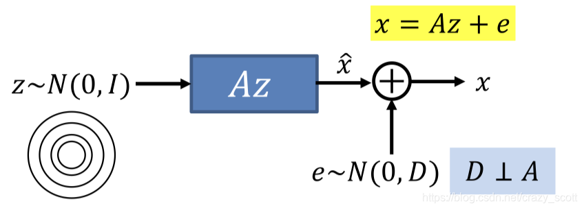
- z ∼ N ( 0 , I ) z \sim N(0, I)z∼N(0,I) => A z AzAz
- The linear transform stretches and rotates the K-dimensional input space onto a Kdimensional hyperplane in the data space
- X = A z + E X = Az +EX=Az+E
- Add Gaussian noise to produce points that aren’t necessarily on the plane
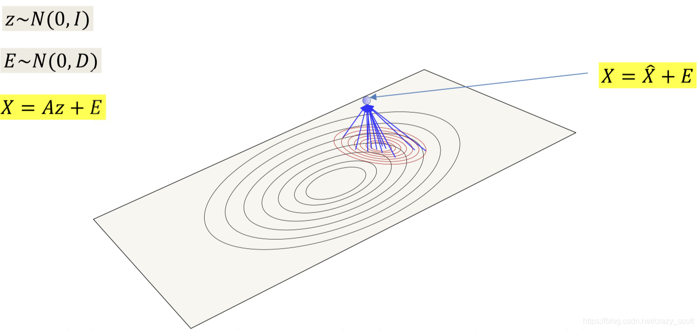
The posterior probability P ( z ∣ x ) P(z|x)P(z∣x) gives you the location of all the points on the plane that could have generated x xx and their probabilities
What about data that are not Gaussian distributed close to a plane?
- Linear Gaussian Models fail
How to do that
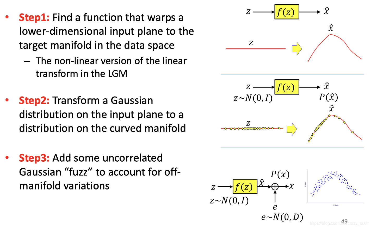
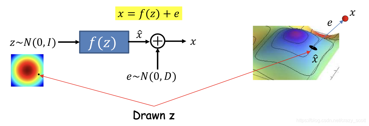
Non-linear Gaussian Model
- f ( z ) f(z)f(z) is a non-linear function that produces a curved manifold
- Like the decoder of a non-linear AE
- Generating process
- Draw a sample z zz from a Uniform Gaussian
- Transform z zz by f ( z ) f(z)f(z)
- This places z zz on the curved manifold
- Add uncorrelated Gaussian noise to get the final observation
- Key requirement
- Identifying the dimensionality K KK of the curved manifold
- Having a function that can transform the (linear) K KK-dimensional input space (space of z zz ) to the desired K KK-dimensional manifold in the data space
With complete data
x = f ( z ; θ ) + e x=f(z ; \theta)+ex=f(z;θ)+e
P ( x ∣ z ) = N ( f ( z ; θ ) , D ) P(x \mid z)=N(f(z ; \theta), D)P(x∣z)=N(f(z;θ),D)
- Given complete information X = [ x 1 , x 2 , … ] , Z = [ z 1 , z 2 , … ] X=\left[x_{1}, x_{2}, \ldots\right], \quad Z=\left[z_{1}, z_{2}, \ldots\right]X=[x1,x2,…],Z=[z1,z2,…]
θ ⋆ , D ⋆ = argmax θ , D ∑ ( x , z ) log P ( x , z ) = argmax θ , D ∑ ( x , z ) log P ( x ∣ z ) \theta^{\star}, D^{\star}=\underset{\theta, D}{\operatorname{argmax}} \sum_{(x, z)} \log P(x, z)=\underset{\theta, D}{\operatorname{argmax}} \sum_{(x, z)} \log P(x \mid z)θ⋆,D⋆=θ,Dargmax(x,z)∑logP(x,z)=θ,Dargmax(x,z)∑logP(x∣z)
= argmax θ , D ∑ ( x , Z ) log 1 ( 2 π ) d ∣ D ∣ exp ( − 0.5 ( x − f ( z ; θ ) ) T D − 1 ( x − f ( z ; θ ) ) ) =\underset{\theta, D}{\operatorname{argmax}} \sum_{(x, Z)} \log \frac{1}{\sqrt{(2 \pi)^{d}|D|}} \exp \left(-0.5(x-f(z ; \theta))^{T} D^{-1}(x-f(z ; \theta))\right)=θ,Dargmax(x,Z)∑log(2π)d∣D∣1exp(−0.5(x−f(z;θ))TD−1(x−f(z;θ)))
= argmax θ , D ∑ ( x , Z ) − 1 2 log ∣ D ∣ − 0.5 ( x − f ( z ; θ ) ) T D − 1 ( x − f ( z ; θ ) ) =\underset{\theta, D}{\operatorname{argmax}} \sum_{(x, Z)}-\frac{1}{2} \log |D|-0.5(x-f(z ; \theta))^{T} D^{-1}(x-f(z ; \theta))=θ,Dargmax(x,Z)∑−21log∣D∣−0.5(x−f(z;θ))TD−1(x−f(z;θ))
- There isn’t a nice closed form solution, but we could learn the parameters using backpropagation
Incomplete data
- The posterior probability is given by
P ( z ∣ x ) = P ( x ∣ z ) P ( z ) P ( x ) P(z \mid x)=\frac{P(x \mid z) P(z)}{P(x)}P(z∣x)=P(x)P(x∣z)P(z)
- The denominator
P ( x ) = ∫ − ∞ ∞ N ( x ; f ( z ; θ ) , D ) N ( z ; 0 , D ) d z P(x)=\int_{-\infty}^{\infty} N(x ; f(z ; \theta), D) N(z ; 0, D) d zP(x)=∫−∞∞N(x;f(z;θ),D)N(z;0,D)dz
- Can not have a closed form solution
- Try to approximate it
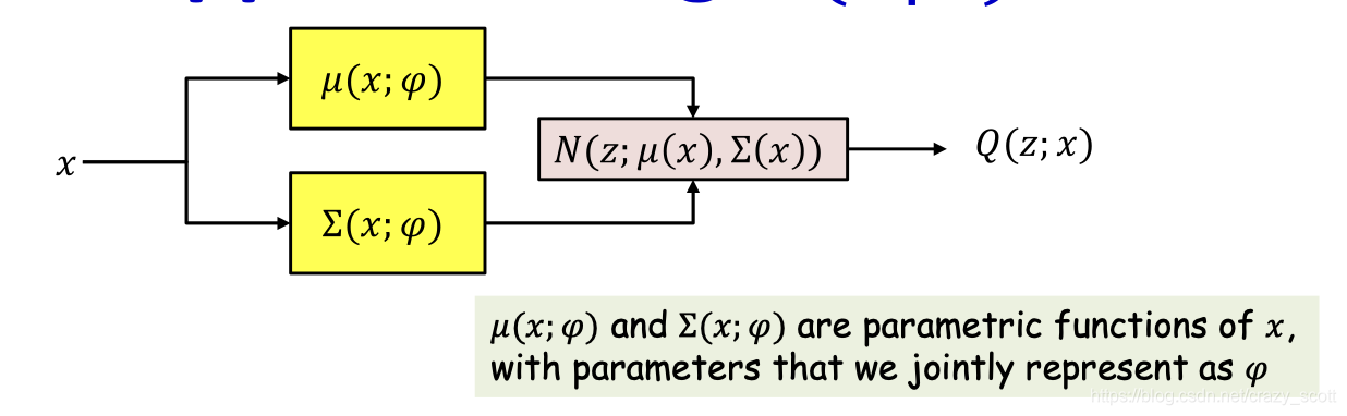
- We approximate P ( z ∣ x ) P(z|x)P(z∣x) as
P ( z ∣ x ) ≈ Q ( z , x ) = Gaussian N ( z ; μ ( x ) , Σ ( x ) ) P(z \mid x) \approx Q(z, x)=\operatorname{Gaussian} N(z ; \mu(x), \Sigma(x))P(z∣x)≈Q(z,x)=GaussianN(z;μ(x),Σ(x))
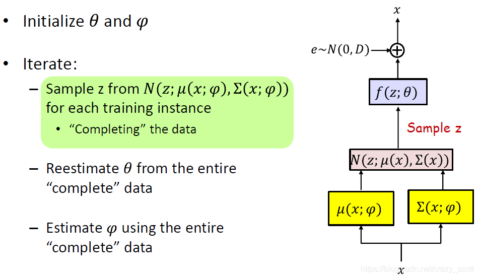
- Sample z zz from N ( z ; μ ( x ; ϕ ) , σ ( x ; ϕ ) ) N(z;\mu (x;\phi),\sigma (x;\phi))N(z;μ(x;ϕ),σ(x;ϕ)) for each training instance
- Draw K KK-dimensional vector ε \varepsilonε from N ( 0 , I ) N(0,I)N(0,I)
- Compute z = μ ( x ; φ ) + Σ ( x ; φ ) 0.5 ε z=\mu(x ; \varphi)+\Sigma(x ; \varphi)^{0.5} \varepsilonz=μ(x;φ)+Σ(x;φ)0.5ε
- Reestimate θ \thetaθ from the entire “complete” data
- Using backpropagation
L ( θ , D ) = ∑ ( x , z ) log ∣ D ∣ + ( x − f ( z ; θ ) ) T D − 1 ( x − f ( z ; θ ) ) L(\theta, D)=\sum_{(x, z)} \log |D|+(x-f(z ; \theta))^{T} D^{-1}(x-f(z ; \theta))L(θ,D)=(x,z)∑log∣D∣+(x−f(z;θ))TD−1(x−f(z;θ))
θ ⋆ , D ⋆ = argmin θ , D L ( θ , D ) \theta^{\star}, D^{\star}=\underset{\theta, D}{\operatorname{argmin}} L(\theta, D)θ⋆,D⋆=θ,DargminL(θ,D)
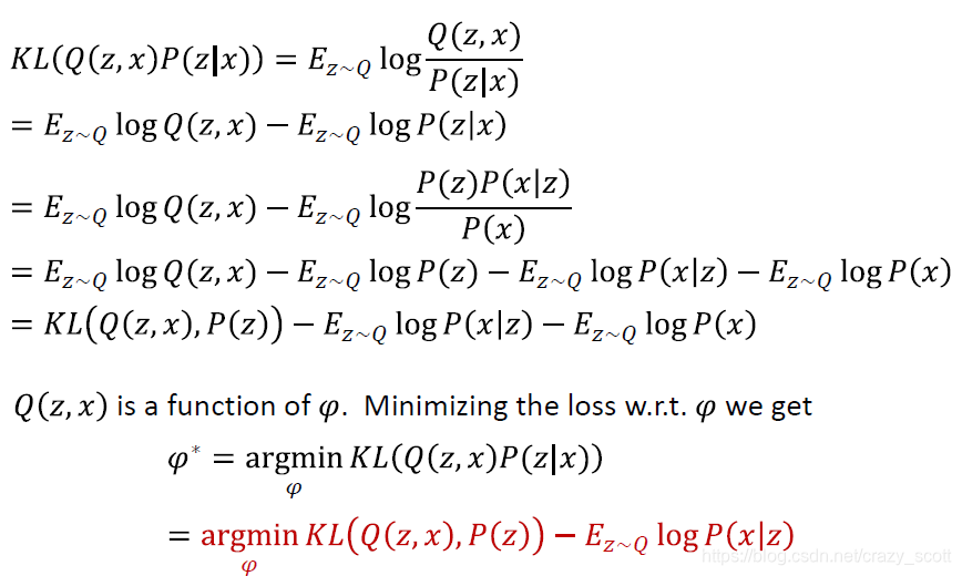
- Estimate φ \varphiφ using the entire “complete” data
- Recall Q ( z , x ) = N ( z ; μ ( x ; φ ) , Σ ( x ; φ ) ) Q(z, x)=N(z ; \mu(x ; \varphi), \Sigma(x ; \varphi))Q(z,x)=N(z;μ(x;φ),Σ(x;φ)) must approximate P ( z ∣ x ) P(z|x)P(z∣x) as closely as possible
- Define a divergence between Q ( z , x ) Q(z,x)Q(z,x) and P ( z ∣ x ) P(z|x)P(z∣x)
Variational AutoEncoder
- Non-linear extensions of linear Gaussian models
- f ( z ; θ ) f(z;\theta)f(z;θ) is generally modelled by a neural network
- μ ( x ; φ ) \mu(x ; \varphi)μ(x;φ) and Σ ( x ; φ ) \Sigma(x ; \varphi)Σ(x;φ) are generally modelled by a common network with two outputs
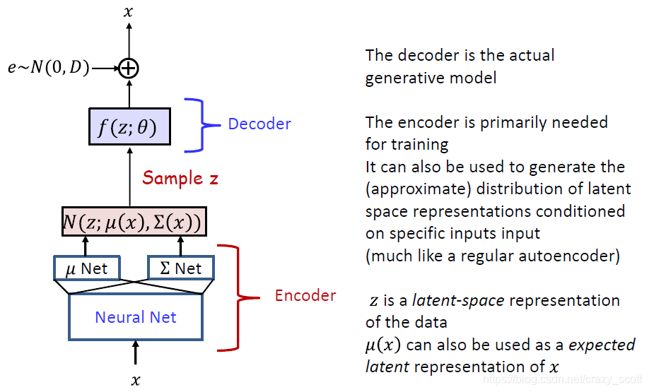
- However, VAE can not be used to compute the likelihoood of data
- P ( x ; θ ) P(x;\theta)P(x;θ) is intractable
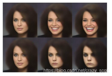
- Latent space
- The latent space z zz often captures underlying structure in the data x xx in a smooth manner
- Varying z zz continuously in different directions can result in plausible variations in the drawn output