算法简介
Isolation Forest算法将分布稀疏,且距离高密度群体较远的点定义为异常点。从统计学角度来看,在数据空间里,若数据点在一个区域内的分布都很稀疏,表示此区域内数据点存在的可能性很小,因此可以认为落在此区域内的数据点都是异常点。由于监控时序数据是连续型结构化数据,异常发生的概率很低,且异常点的特征值与正常点的特征值差异很大,所以适合用Isolation Forest 算法进行异常检测。隔离森林属于无监督异常检测算法。
算法流程
隔离森林是由多棵树组成的,其基本思想是
- 随机选取一个特征,并从样本中随机选取一个值,建立树,对于随机选取的一个值P,当前节点的左分支存放小于p所选维度的数据点,当前节点的右分支存放大于或等于p所选维度的数据点;
- 递归的不断构造树,直到所有样本都在树中,或者树的高度达到了指定值。对于那些异常的点可以认为其很早的就会被分到叶子节点,故计算每个节点到根节点的距离,计算路径长度。
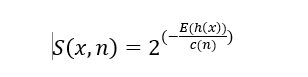
- 建立多棵隔离树,计算每个特征值的平均路径长度。根据孤立森林的异常分数计算公式,计算每个样本数据其中n为样本数,二叉搜索树的平均路径长度。计算公式如下
sklearn isolation forest实现
- 导入sklearn的包
from sklearn.ensemble import IsolationForest
from sklearn.ensemble import _iforest
- 建立隔离森林模型
clf = IsolationForest(max_samples=n_samples, random_state=rng, contamination='auto',max_features=12,n_estimators=50)
参数说明
max_samples:用于建立树的样本数量
random_state: 随机数种子,用于重现模型
contamination:异常样本的百分比,在[0,0.5]之间的float型,默认为0.5
max_features:特征数——用于训练的数据可以是多维的
n_estimators:建立隔离树的数量,一般默认为100
clf为建立的隔离森立的模型
-
clf.fit(X_train)
使用数据集X_train来训练模型,使用fit函数
-
y_pred_train = clf.predict(X_train)
查看隔离森林得出的结果,输出为一维矩阵,其中值为1代表为正常数据点,值为-1代表为异常点
-
alv = _iforest._average_path_length(X_train)
查看数据中每个样本的平均路径长度
-
score = clf.decision_function(X_train)
数据集中样本的异常分数值,注意其中值是以0为阈值,小于0视为异常,大于0视为正常,其内部实现返回的是
self.score_samples(X) -self.offset_
-
_compute_chunked_score_samples
这才是正真实现了原论文中的异常分数的计算,由于原论文中没有提到阈值是多少,所以在sklearn中是根据contamination的值来确定异常样本的比例来计算阈值
也就是跟self.offset_函数相关,具体实现
        if self.contamination == "auto":
            # 0.5 plays a special role as described in the original paper.
            # we take the opposite as we consider the opposite of their score.
            self.offset_ = -0.5
            return self

        # else, define offset_ wrt contamination parameter
        self.offset_ = np.percentile(self.score_samples(X),
                                     100. * self.contamination)
默认为 -0.5,np.percentile为百分位数是统计中使用的度量,表示小于这个值的观察值的百分比。 函数numpy.percentile()接受以下参数。
numpy.percentile(a,q,axis)参数说明:
- a: 输入数组
- q: 要计算的百分位数,在 0 ~ 100 之间
- axis: 沿着它计算百分位数的轴
具体实现sklearn官方的实例
import numpy as np
import matplotlib.pyplot as plt
from sklearn.ensemble import IsolationForest
# 随机数相关,后期用来构造测试数据
rng = np.random.RandomState(42)
# Generate train data
# 生成100行2列array的0-1随机数,并且乘0.3,映射值域到[0,0.3]
X = 0.3 * rng.randn(100, 2)
# 对X分别加减2,得到两个(100,2)的矩阵
# 通过np.r_,对两个矩阵行合并,类似R里的rbind
X_train = np.r_[X + 2, X - 2]
# Generate some regular novel observations
# 下面生成测试数据,分布和生成逻辑保持一致
X1 = 0.3 * rng.randn(20, 2)
X_test = np.r_[X1 + 2, X1 - 2]
# Generate some abnormal novel observations
# 异常值由均匀分布U(-4,4)构造,20行2列的array
X_outliers = rng.uniform(low=-4, high=4, size=(20, 2))
# fit the model
clf = IsolationForest(max_samples=100, random_state=rng)
clf.fit(X_train)
y_pred_train = clf.predict(X_train)
y_pred_test = clf.predict(X_test)
y_pred_outliers = clf.predict(X_outliers)
print("------ _compute_score_samples ------"+"\n");print(clf._compute_score_samples(np.asarray(X),False)[1:10])
print("------ _compute_chunked_score_samples ------"+"\n");print(clf._compute_chunked_score_samples(np.asarray(X))[1:10])
print("------ score_samples ------"+"\n");print(clf.score_samples(X)[1:10])
print("------ decision_function ------"+"\n");print(clf.decision_function(X)[1:10])
# plot the line, the samples, and the nearest vectors to the plane
#
xx, yy = np.meshgrid(np.linspace(-5, 5, 50), np.linspace(-5, 5, 50))
# xx.ravel()转成1维
# np.c_列拼接cbind
Z = clf.decision_function(np.c_[xx.ravel(), yy.ravel()])
# 重塑
Z = Z.reshape(xx.shape)
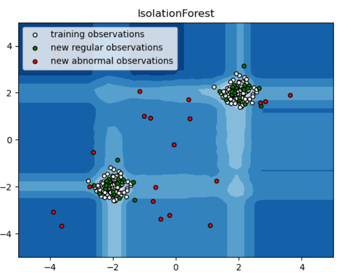
plt.title("IsolationForest")
plt.contourf(xx, yy, Z, cmap=plt.cm.Blues_r)
# 白色的点为train
b1 = plt.scatter(X_train[:, 0], X_train[:, 1], c='white',
s=20, edgecolor='k')
# 绿色的点为test
b2 = plt.scatter(X_test[:, 0], X_test[:, 1], c='yellow',
s=20, edgecolor='k')
# 红色点为outliers
c = plt.scatter(X_outliers[:, 0], X_outliers[:, 1], c='red',
s=20, edgecolor='k')
plt.axis('tight')
plt.xlim((-5, 5))
plt.ylim((-5, 5))
plt.legend([b1, b2, c],
["training observations",
"new regular observations", "new abnormal observations"],
loc="upper left")
plt.show()
实现图如下