还是老规矩先宣传一下QQ群群: 格子玻尔兹曼救星:293267908。免费群!一切为了早日毕业。
最近群友问画图的挺多,动态图,伪色彩图、矢量图、流线图,散点图折线图。。我在这里贡献一下自己的MATLAB画图代码算是给大家提供参考。
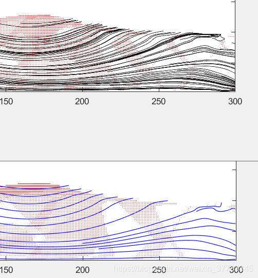
- 1 流线图。
用任何语言生成的xy坐标和uv速度场,怎么画流线图和矢量图呢,MATLAB提供streamslice函数:
%From  https://ww2.mathworks.cn/help/matlab/ref/streamslice.html
hh=streamslice(ux',uy','k','noarrows');axis equal off; drawnow;
set(hh, 'Color', 'black');
那么复杂一点呢,可以这样:
%text= load('your_velocitydata.txt'); %load your data
% x=text(:,1);
% r=text(:,2);
% dvx=text(:,3);
% dvr=text(:,4);

%xy Range : 如果workplace就有数据矩阵,直接用就行,不用load:
cor_inix=1;cor_finx=300;
cor_iniy=1;cor_finy=100;

coum=0;
x=[];
r=[];
dvx=[];
dvr=[];
for j=cor_iniy:cor_finy
    for i=cor_inix:cor_finx
        coum=coum+1;
        x(coum,1)=i;
        r(coum,1)=j;
        dvx(coum,1)=ux(i,j);
        dvr(coum,1)=uy(i,j);
    end
end
%[xs,rs] = meshgrid(x,r);

Fx = scatteredInterpolant(x,r,dvx);  %对数据集执行插值
Fr = scatteredInterpolant(x,r,dvr);
%
xx=linspace(min(x),max(x),90);      % xx= linspace(x1,x2,n) 生成 n 个点。这些点的间距为 (x2-x1)/(n-1)。 调节此处可以调整疏密度!
rr=linspace(min(r),max(r),90);%n control the streamline beyound the free surface
[xgg,rgg]=meshgrid(xx,rr);
xstream = Fx(xgg,rgg);
ystream = Fr(xgg,rgg);
%
scrsz = get(0,'ScreenSize');         %得到屏幕参数

figure1 = figure('Position',[0.06*scrsz(3) 0.06*scrsz(4) 0.5*scrsz(3) 0.5*scrsz(4)]);   % 改变画图大小位置
                                     % scrsz(1): 屏幕最左坐标;scrsz(2): 屏幕最下坐标
                                     % scrsz(3): 屏幕宽(像素);% scrsz(4): 屏幕高(像素)
% [xs,rs] = meshgrid(x,r); %[dvxs,dvrs] = meshgrid(dvx,dvr);

quiver(x,r,dvx,dvr,'r'); %Important!! meng

numstream=250; % number of lines
strx=randi([cor_inix,cor_finx],numstream,1);       %randi([imin,imax],...) 返回一个在[imin,imax]范围内的伪随机整数
stry=randi([cor_iniy,cor_finy],numstream,1);       %r = randi(imax,[m,n]),返回一个在[1,imax]范围内的的m*n的伪随机整数矩阵 原始为stry=randi([0,12],numstream,1);
                                      %值strx、y代表流线的起始位置
strx=[strx,strx];
stry=[stry,-stry];

h=streamline(xgg,rgg,xstream,ystream,strx,stry); %streamline(X,Y,Z,U,V,W,startx,starty,startz) 根据三维向量数据 U、V 和 W 绘制流线图。
                                                 %数组 X、Y 和 Z 用于定义 U、V 和 W 的坐标,它们必须是单调的,无需间距均匀。X、Y 和 Z 必须具有相同数量的元素,就像由 meshgrid 生成一样。
                                                 %startx、starty 和 startz 定义流线图的起始位置。

set(h,'LineWidth',0.5,'Color','k')

axis equal
axis tight
box on

%  2nd
figure2 = figure('Position',[0.06*scrsz(3) 0.06*scrsz(4) 0.6*scrsz(3) 0.6*scrsz(4)]);% Call a picture. 0.5*scrsz(3):size.

% [xs,rs] = meshgrid(x,r);%[dvxs,dvrs] = meshgrid(dvx,dvr);

%quiver(x,r,dvx,dvr,'r');

numstream=500;
strx=randi([cor_inix,cor_finx],numstream,0);
stry=randi([cor_iniy,cor_finy],numstream,0);         %此处原为[0,12]

strx=[strx,strx];
stry=[stry,-stry];

h=streamslice(xgg,rgg,xstream,ystream,'noarrows');  %流线图
%h=streamslice(xgg,rgg,xstream,ystream);  %流线图, with arrows
set(h,'LineWidth',0.7,'Color','b')

axis equal
axis tight
box on看!大波~!浪!

放错了。再来,大波~浪!
- 2 色彩图
%Draw picture
%初始设置,xDim,yDim 是你的横纵网格的数目
[meshX,meshY]=meshgrid(1:xDim,yDim:-1:1);% in MATLAB,we have to change the orderof y
figure %Summon picture
pc=pcolor(meshX,meshY,ones(yDim,xDim));%Pseudo color image
shading interp%shading interp:It will distinguish the color of each linear area, and insert the color similar to it
%axis equal
ylim([1 yDim])  %y-axis upper and lower limit setting
title('Russell test 04: ParDen=1.25, tau=0.505, xgap=0.025, qgravity=-9.3e-05, xDim=9m')

%主循环:算出速度场u2,v2...

%后处理
u2=rot90(u1); % 用前 扭一扭
v2=rot90(v1);
        for i=1:xDim
            for j=1:yDim
                speed(j,i)=sqrt(u2(j,i)^2+v2(j,i)^2);%resultant v
            end
        end
        set(pc,'cdata',speed);
        drawnow
        pbaspect([25 1 1]) % order: L=H
        %axis equal
        ylim([1 yDim])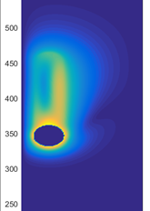
- 3、画压力或者速度场:
for j=fix(x0_p-R-5):fix(x0_p+R+5)
    for i=fix(y0_p-R-5):fix(y0_p+R+5)
        if bc(i,j)==-1
            p(i,j)= 0.3336 ;%这个赋值 是由于这个区域是个固体,所以我随意给了个数值,否则压力和周边流体差异过大,不容易显示出来细微的压力变化。不信你去掉这个for循环就行。
        end
    end
end
figure
contourf(1:X ,1:Y,p)
axis equal
%title('压力场')
ylim([1 Y])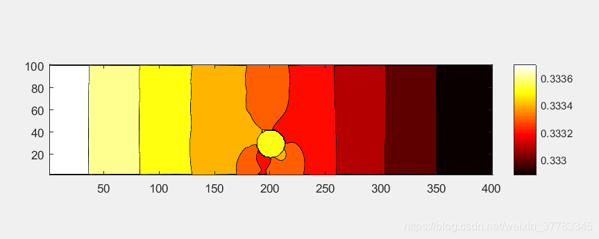
右击图例可以修改各种效果。
%MATLAB图像处理: m2020/3/13
figure
uv=sqrt(ux.^2+uy.^2);
contourf(1:X ,1:Y,uv)
axis equal
%title('模型的速度场')
ylim([1 Y])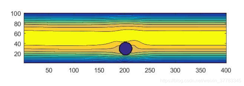
当然也可以直接 imagesc(rho); axis equal;
再来一个画密度的例子。
 figure
        x = linspace(0,1000,n+1)';
        y = linspace(0,40,m+1)';
        [X, Y] = meshgrid(x,y);

        contourf(X, Y, rho',20);
        colorbar;
        xlabel('x');
ylabel('y');- 4、Gif图。一直都在用这个。推荐给大家。
%clc;clear all;close all;
firstpic=25;%第一个图片的编号
%num_image = 8;
dst_dir = 'E:\matlabwork\.....test 03\'; %图片的位置:注意最后一定要有这个 \

filename= 'test 03.gif'; %你的gif文件的名字
for i=firstpic:Step2:cycle % Step2 是图片编号的间隔,cycle 是最后一个图片的编号
    idx=sprintf('%d',i);
    str=[dst_dir idx '.jpg']; %打开每个图片的名字
    Img=imread(str);
    figure(i)
    imshow(Img);
    frame=getframe(i);
    im=frame2im(frame);%制作gif文件,图像必须是index索引图像
    [I,map]=rgb2ind(im,256);
     if i==firstpic
        imwrite(I,map,filename,'gif','Loopcount',inf,'DelayTime',0.1);     %Loopcount只是在i==1的时候才有用
    else
        imwrite(I,map,filename,'gif','WriteMode','append','DelayTime',0.2);%DelayTime:帧与帧之间的时间间隔
    end
end
close all- 5、散点和折线图:
以几个质点水平速度ux随着时间步变化的曲线为例:
%画图:
i0=100;%自变量初始值
ig=100;%自变量取值间隔
ini=10000;%自变量最大值
load('E:\matlabwork\...\workspace1.mat') %加载某个数据文件
plot(ux_p(i0:ig:ini),'ko-','LineWidth',1);%ux_p是一个数列,是因变量。k是黑色,带圆圈的折线图。'ko'是散点图。'LineWidth'=1
hold on ;%下一个图
load('E:\matlabwork\...\workspace12.mat')
plot(ux_p(i0:ig:ini),'k+','LineWidth',1); % 散点图
hold on ;
%....以此类推,'k.-','k-'等

%自动依次加标签:
legend('test H=0.001','test H=-0.001',... ); % legend 会自动根据画图顺序分配图形
xlabel('时间步(单位)','Fontsize',18);ylabel('水平速度(ux)','Fontsize',18);
hold off ;
补充:更换MATLAB的储存位置和加载数据:
cd C:\Users\...%你的地址;
load workspace1.mat;%地址里的数据- 6、转成tecplot,这个有个哥们写了,直接推荐给大家:
1: https://blog.csdn.net/weixin_42943114/article/details/104204172
2:https://www.cnblogs.com/zhubinglong/p/8735426.html
3:https://wenku.baidu.com/view/70b794168e9951e79a892721.html?from=search
4:http://www.doc88.com/p-618423100007.html
这个是适用于MATLAB-tecplot的函数例子,用于生成.dat文件:
function result(nx,ny,u,v,obst,count,uo)
pi=0;
Uz=(u.^2+v.^2).^0.5;
xn=[1:nx]'; yn=[1:ny]';
for i=1:nx
    for j=1:ny
        if obst(i,j)==1
            u(i,j)=0; v(i,j)=0; Uz(i,j)=0;
        end
        pi=pi+1;
        peess(pi,:)=[xn(i),yn(j),u(i,j)/uo,v(i,j)/uo,Uz(i,j)/uo];
    end
end
filename=['F:\LBM_code\date-2\' num2str(count) '-tecplot2d.dat'];
%   address是储存位置,这里的num2str是为了在循环输出dat数据文件中使用,如果只有一个文件可以忽略
fid=fopen(filename,'wt');
fprintf(fid,'variables= "x", "y", "U", "V", "Uz"\n');
fprintf(fid,'zone t="Frame 0"i=%d,j=%d,f=point\n',ny,nx);
fprintf(fid,'SOLUTIONTIME=%d\n',count);
fprintf(fid,'%8.4f %8.4f %8.4f %8.4f %8.4f\n',peess');
fclose(fid);
end
版权声明:本文为weixin_37783345原创文章,遵循CC 4.0 BY-SA版权协议,转载请附上原文出处链接和本声明。