线性回归算法原理的梳理过程

线性回归算法原理的梳理过程

概念

1.有监督
2.线性
3.模型 函数

import numpy as np
import matplotlib.pyplot as plt

数据预处理的过程

x = np.array([4, 3, 3, 4, 2, 2, 0, 1, 2, 5, 1, 2, 5, 1, 3])
y = np.array([8, 6, 6, 7, 4, 4, 2, 4, 5, 9, 3, 4, 8, 3, 6])
m = len(x)#获取样本的数量
#x增加一列1
x = np.c_[np.ones([m, 1]), x]
print(x.shape)
#为了后续维度对应，y也做维度变化
y = y.reshape(15, 1)
print(y.shape)

(15, 2)
(15, 1)

theta 的值是随机创建

theta = np.zeros([2, 1])
print(theta)

[[ 0.]
 [ 0.]]

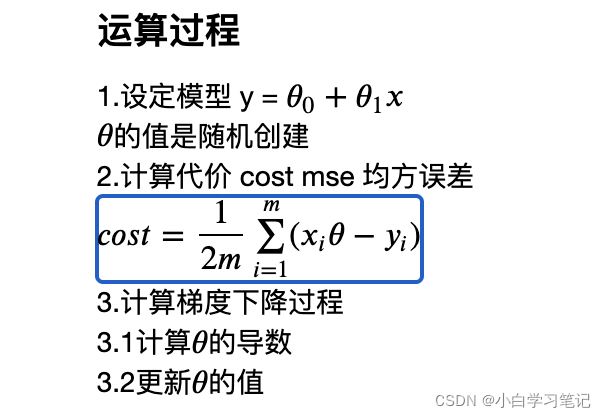
1.设定模型 $ \hat{y} = \theta_0 + \theta_1 x$
2.计算代价 cost mse 均方误差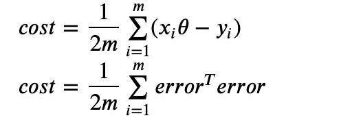

3.计算梯度下降过程
3.1计算$\theta
$的导数
$\Delta \theta =\frac{1}{m}{x}^{T}error$
3.2更新$\theta$的值
$\theta :=\theta -\alpha \Delta \theta$

# 超参数alpha 学习率  步长
alpha = 0.01
#迭代次数
m_iter = 1000
#定义一个数组，存储所有的代价数据
cost = np.zeros([m_iter])
for i in range(m_iter):
    y_hat = x.dot(theta)#求预测值
    error = y_hat - y #误差值
    cost_val = 1 / 2 * m *error.T.dot(error)#代价值
    cost[i] = cost_val#记录代价值
    delta_theta = 1 / m * x.T.dot(error)#求导数
    theta = theta - alpha * delta_theta#更新参数
print(theta)

[[ 1.70993385]
 [ 1.39189459]]

#使用图形进行演示
plt.scatter(x[:,1], y, c='blue')# x有两列数据
plt.plot(x[:, 1], y_hat, 'r-')#预测模型
plt.show()

#代价值的显示
plt.plot(cost)
plt.show()