python全景拼接
简述流程:RANSAC算法矫正-->计算单应性矩阵-->特征点匹配-->图片匹配-->图像拼接
(一)环境说明
pyhton版本为3.7、使用脚本为IDLE编译、vlfeat版本为vlfeat-0.9.20
下载vlfeat-0.9.20链接:https://pan.baidu.com/s/1MbIhHyy2AurektPJQJb11g
提取码:oohd
复制这段内容后打开百度网盘手机App,操作更方便哦
(二)全景拼接原理描述
1.稳健的单应性矩阵估计(RANSAC算法):通过测试得到并不是所有的匹配图片中对应的匹配点都是正确的。虽然使用的是sift算法进行特征匹配,sift又具有很强的稳健性,不会因光照、旋转、平移、尺度等因素的改变而消失。虽然很少产生错误点,但是并非非常完美,也会出现拼接错误。
sift原理请看此链接:https://blog.csdn.net/weixin_43837871/article/details/88604483
单应性变换请看此连接:https://blog.csdn.net/weixin_43837871/article/details/88669826

为了纠正错误匹配点而导致不正确拼接,RANSAC(随机一致性采样)就能很好的解决这个问题。该方法是用来找到正确模型来拟合带有噪声数据的迭代方法,数据中包含正确的点和噪声点。RANSAC优点之处:用一条直线拟合带有噪声数据的点集合,最简单的最小二乘法可能会失效;但是RANSAC却能够挑出正确的点,摒弃错误的点。

如何计算单应性矩阵:只要用python实现相应的fit()和get_error()方法和正确使用ransac.py文件就可以的到相应的单应性矩阵。本博文采用的是对应点自动找到用于全景图像的单应性矩阵。
from pylab import *
from numpy import *
from PIL import Image

# If you have PCV installed, these imports should work
from PCV.geometry import homography, warp
import sift

featname = ['E:/Python37_course/test2/test'+str(i+1)+'.sift' for i in range(5)]
imname = ['E:/Python37_course/test2/test'+str(i+1)+'.jpg' for i in range(5)]

l = {}
d = {}
for i in range(5):
    sift.process_image(imname[i],featname[i])
    l[i],d[i] = sift.read_features_from_file(featname[i])

matches = {}
for i in range(4):
    matches[i] = sift.match(d[i+1],d[i])
for i in range(4):
    im1 = array(Image.open(imname[i]))
    im2 = array(Image.open(imname[i+1]))
    figure()
    sift.plot_matches(im2,im1,l[i+1],l[i],matches[i],show_below=True)


# function to convert the matches to hom. points
def convert_points(j):
    ndx = matches[j].nonzero()[0]
    fp = homography.make_homog(l[j+1][ndx,:2].T)
    ndx2 = [int(matches[j][i]) for i in ndx]
    tp = homography.make_homog(l[j][ndx2,:2].T)

    # switch x and y - TODO this should move elsewhere
    fp = vstack([fp[1],fp[0],fp[2]])
    tp = vstack([tp[1],tp[0],tp[2]])
    return fp,tp
我们可以从homography.py文件里看出,这个类就包含了fit()方法,这种方法只接受ransac.py选择的4个对应点对(data中前四个点对,是计算单应性矩阵所需要的最少数目),然后合成一个单应性矩阵。get_error()方法是对每一个对应点对使用该单应性矩阵,之后返回相对应的平房距离之和(实际过程中需要在距离上使用一个阈值来决决定哪些单应性矩阵是合理的)。所以,RANSAC算法能够判断出哪些点对是正确的,哪些点对是错误的。
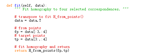

 该函数允许提供阈值和最小期望值的点对数目。最重要的是最大迭代次数:退出太早可能会得到坏解,太多又会浪费时间。
对应的 H:

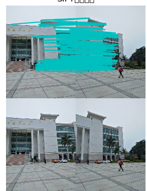
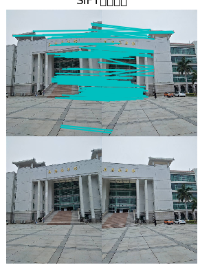
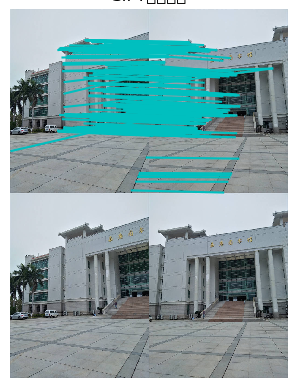
2.进行sift特征点匹配,得到结果:

3.拼接图像
图片拼接就是估计出图像间的单应性矩阵(用RANSAC算法得出),然后将所有的图像扭曲到一个公共的图像平面上。而公共平面通常为中心图像平面。本博文采用的方法是创建一个很大的图像,全部以0填充(简单步骤:将中心图像左边或右边的区域填充0,以便于为扭曲的图像腾出空间),然后使其和中心图像平行,再将所有的图像扭曲到上面。
在wrap.py文件中,使用transf()函数指定能够描述像素到像素间映射关系,该函数通过将像素和H相乘,然后对齐次坐标进行归一化实现像素间的映射。再通过查看H中的平移量决定将图片填补在左边还是右边,由于目标图像坐标再变化,为了简单起见,使用0像素寻找alpha。最后因为图像曝光不同,可以进行简单的平滑场景转换,可以达到更好的效果
(三)实现全景拼接
sift.py
from PIL import Image
import os
from numpy import *
from pylab import *


def process_image(imagename, resultname, params="--edge-thresh 10 --peak-thresh 5"):
    """ 处理一幅图像,然后将结果保存在文件中"""

    if imagename[-3:] != 'pgm':
        #创建一个pgm文件
        im = Image.open(imagename).convert('L')
        im.save('tmp.pgm')
        imagename ='tmp.pgm'
    cmmd = str(r"E:\Python37_course\test2\sift.exe "+imagename+" --output="+resultname+" "+params)
   # cmmd = str("sift "+imagename+" --output="+resultname+" "+params)
    os.system(cmmd)
    print ('processed', imagename, 'to', resultname)


def read_features_from_file(filename):
    """读取特征属性值,然后将其以矩阵的形式返回"""
    f = loadtxt(filename)
    return f[:,:4], f[:,4:] #特征位置,描述子

def write_featrues_to_file(filename, locs, desc):
    """将特征位置和描述子保存到文件中"""
    savetxt(filename, hstack((locs,desc)))

def plot_features(im, locs, circle=False):
    """显示带有特征的图像
       输入:im(数组图像),locs(每个特征的行、列、尺度和朝向)"""

    def draw_circle(c,r):
        t = arange(0,1.01,.01)*2*pi
        x = r*cos(t) + c[0]
        y = r*sin(t) + c[1]
        plot(x, y, 'b', linewidth=2)

    imshow(im)
    if circle:
        for p in locs:
            draw_circle(p[:2], p[2])
    else:
        plot(locs[:,0], locs[:,1], 'ob')
    axis('off')


def match(desc1, desc2):
    """对于第一幅图像中的每个描述子,选取其在第二幅图像中的匹配
    输入:desc1(第一幅图像中的描述子),desc2(第二幅图像中的描述子)"""
    desc1 = array([d/linalg.norm(d) for d in desc1])
    desc2 = array([d/linalg.norm(d) for d in desc2])

    dist_ratio = 0.6
    desc1_size = desc1.shape
    matchscores = zeros((desc1_size[0],1),'int')
    desc2t = desc2.T #预先计算矩阵转置
    for i in range(desc1_size[0]):
        dotprods = dot(desc1[i,:],desc2t) #向量点乘
        dotprods = 0.9999*dotprods
        # 反余弦和反排序,返回第二幅图像中特征的索引
        indx = argsort(arccos(dotprods))

        #检查最近邻的角度是否小于dist_ratio乘以第二近邻的角度
        if arccos(dotprods)[indx[0]] < dist_ratio * arccos(dotprods)[indx[1]]:
            matchscores[i] = int(indx[0])

    return matchscores


def match_twosided(desc1, desc2):
    """双向对称版本的match()"""
    matches_12 = match(desc1, desc2)
    matches_21 = match(desc2, desc1)

    ndx_12 = matches_12.nonzero()[0]

    # 去除不对称的匹配
    for n in ndx_12:
        if matches_21[int(matches_12[n])] != n:
            matches_12[n] = 0

    return matches_12


def appendimages(im1, im2):
    """返回将两幅图像并排拼接成的一幅新图像"""
    #选取具有最少行数的图像,然后填充足够的空行
    rows1 = im1.shape[0]
    rows2 = im2.shape[0]

    if rows1 < rows2:
        im1 = concatenate((im1, zeros((rows2-rows1,im1.shape[1]))),axis=0)
    elif rows1 >rows2:
        im2 = concatenate((im2, zeros((rows1-rows2,im2.shape[1]))),axis=0)
    return concatenate((im1,im2), axis=1)


def plot_matches(im1,im2,locs1,locs2,matchscores,show_below=True):
    """ 显示一幅带有连接匹配之间连线的图片
        输入:im1, im2(数组图像), locs1,locs2(特征位置),matchscores(match()的输出),
        show_below(如果图像应该显示在匹配的下方)
    """
    im3=appendimages(im1,im2)
    if show_below:
        im3=vstack((im3,im3))
    imshow(im3),title('SIFT特征匹配')

    cols1 = im1.shape[1]
    for i in range(len(matchscores)):
        if matchscores[i]>0:
            plot([locs1[i,0],locs2[matchscores[i,0],0]+cols1], [locs1[i,1],locs2[matchscores[i,0],1]],'c')
    axis('off')
test.py
from pylab import *
from numpy import *
from PIL import Image

# If you have PCV installed, these imports should work
from PCV.geometry import homography, warp
import sift

"""
This is the panorama example from section 3.3.
"""

# set paths to data folder
featname = ['E:/Python37_course/test2/test'+str(i+1)+'.sift' for i in range(5)]
imname = ['E:/Python37_course/test2/test'+str(i+1)+'.jpg' for i in range(5)]

# extract features and match
l = {}
d = {}
for i in range(5):
    sift.process_image(imname[i],featname[i])
    l[i],d[i] = sift.read_features_from_file(featname[i])

matches = {}
for i in range(4):
    matches[i] = sift.match(d[i+1],d[i])

# visualize the matches (Figure 3-11 in the book)
for i in range(4):
    im1 = array(Image.open(imname[i]))
    im2 = array(Image.open(imname[i+1]))
    figure()
    sift.plot_matches(im2,im1,l[i+1],l[i],matches[i],show_below=True)


# function to convert the matches to hom. points
def convert_points(j):
    ndx = matches[j].nonzero()[0]
    fp = homography.make_homog(l[j+1][ndx,:2].T)
    ndx2 = [int(matches[j][i]) for i in ndx]
    tp = homography.make_homog(l[j][ndx2,:2].T)

    # switch x and y - TODO this should move elsewhere
    fp = vstack([fp[1],fp[0],fp[2]])
    tp = vstack([tp[1],tp[0],tp[2]])
    return fp,tp


# estimate the homographies
model = homography.RansacModel()

fp,tp = convert_points(1)
H_12 = homography.H_from_ransac(fp,tp,model)[0] #im 1 to 2

fp,tp = convert_points(0)
H_01 = homography.H_from_ransac(fp,tp,model)[0] #im 0 to 1

tp,fp = convert_points(2) #NB: reverse order
H_32 = homography.H_from_ransac(fp,tp,model)[0] #im 3 to 2

tp,fp = convert_points(3) #NB: reverse order
H_43 = homography.H_from_ransac(fp,tp,model)[0] #im 4 to 3


# warp the images
delta = 700 # for padding and translation

im1 = array(Image.open(imname[1]), "uint8")
im2 = array(Image.open(imname[2]), "uint8")
im_12 = warp.panorama(H_12,im1,im2,delta,delta)

im1 = array(Image.open(imname[0]), "f")
im_02 = warp.panorama(dot(H_12,H_01),im1,im_12,delta,delta)

im1 = array(Image.open(imname[3]), "f")
im_32 = warp.panorama(H_32,im1,im_02,delta,delta)

im1 = array(Image.open(imname[4]), "f")
im_42 = warp.panorama(dot(H_32,H_43),im1,im_32,delta,2*delta)


figure()

imshow(array(im_42, "uint8"))
axis('off')

show()
(1)室外落差不大的场景(5张)
运行结果:

如果出现上面情况,是因为在test.py文件中用于填充平移的数值(delta = 700 # for padding and translation)给的太大,改小一些就可以得到下面结果。(也可以对图片进行中间部分裁剪再显示)

对于室外落差不大的场景拼接,同一个方位,拍摄旋转角度不大,而且没有场景落差大的建筑物影响,而且相似的像素点比较少,RANSAC算法能够很好筛选错误点对,所以效果不错,拼接的折痕不明显,没有出现鬼影现象。但是图片之间有时会有一点曝光差,即使同一时间同一地点同样拍摄设备,也会有些影响。
(2)室内场景拼接(4张)


以上室内全景拼接出现像素点失真,是因为我的图片像素压缩太小而导致的,而出现鬼影,是因为室内的地面和玻璃像素点很相似,且地面的倒影出现鬼影现象,多是因为计算机不能跟人眼一样能分辨出倒影内容是对是错,只是根据图片的像素矩阵判断是否相同,所以会出现较大误差,导致拼接出现鬼影。所以目前图像匹配最大的难点就是玻璃及光滑地面反射的倒影如何判断是否是同一物体。
(四)出现的问题
(1)如果在sift特征匹配出现错误:OSError: E:/Python37_course/test2/Univ1.sift not found.
注释:前段时间写图片分类和sift特征匹配的时候这个问题已经解决,可是在运行全景拼接的时候又出现无法生成.sift文件,以致于出现找不到这个.sift错误。
这个问题的解决方法:就是重新创建一个项目,把对应的py文件和所有图片放在里面。把vlfeat-0.9.20里的sift.exe和vl.dll vl.lib放到项目里:这几个文件所在路径:E:\360Downloads\vlfeat-0.9.20\bin\win64

(1)没有导入PCV的情况,新建一个sift.py文件,把里面读取sift.exe的路径改一下:cmmd = str(r"E:\Python37_course\test2\sift.exe "+imagename+" --output="+resultname+" "+params)

(2)导入了PCV情况,同以上方法该路径,例如:我的PCV的sift.py文件的路径在:D:\Python37\Lib\site-packages\PCV\localdescriptors。但是我建议,自己新建一个新的sift.py文件方法更好,以便于之后编码其他情况可以正常运行。

(2)出现错误:ValueError: did not meet fit acceptance criteria

这是因为这段代码在计算单应性矩阵时,每个图像对中,匹配是从最右边的图像计算出来的,如果你的第二张与第一张图片没有共同点,会错乱拼接图片或者出现ValueError: did not meet fit acceptance criteria错误。所以你在给图片命名时,要按照从右到左的顺序命名。
图片资源
在用自己拍摄的图片进行测试的时,需要相对把图片压缩小一点,按照一定的宽度自适应高度或者按照一定的高度自适应宽度都可以。以致于运行时会快一些,而且不会出现数组溢出党的错误。
相关代码+图片下载连接:https://pan.baidu.com/s/1VJUJdfVIQxvzDXqjUCx6eg
提取码:m9zz

