导包

import numpy as np
import os
import matplotlib.pyplot as  plt
%matplotlib inline

定义保存图像的函数

#随机种子
np.random.seed(42)

#保存图像
PROJECT_ROOT_DIR ='.'
MODEL_ID ='linear_models'

def save_fig(fig_id, tight_layout = True):#定义一个保存图像的函数
    path = os.path.join(PROJECT_ROOT_DIR, 'images',MODEL_ID, fig_id +'.png')#指定保存图像的路径 当前目录下的images文件夹下的model_id文件夹
    print("Saving figure", fig_id) #提示函数，正在保存图片
    print('Saving figure',fig_id)#提示函数
    plt.savefig(path, format='png', dpi =300)#保存图片（需要指定保存路径，保存格式，清晰度）
 # './images/linear_models/xx.png'
# 把讨厌的警告信息过滤掉
import warnings
warnings.filterwarnings(action = 'ignore',message='internal gelsd')

生成训练数据

import numpy as np
x = 2*np.random.rand(100,1) #生成训练数据(特征部分)
y = 4+3*x+np.random.randn(100,1)#生成训练数据(标签部分)

画图

plt.plot(x,y, 'b.')#画图
plt.xlabel('$x_1$',fontsize =18)
plt.ylabel('$y$',rotation=0, fontsize =18)
plt.axis([0,2,0,15])
save_fig('generated_data_plot')# 保存图片

结果：

Saving figure generated_data_plot

添加新特征

#添加新特征
x_b = np.c_[np.ones((100,1)),x]
x_b

结果：

array([[1. , 0.74908024],
[1. , 1.90142861],
[1. , 1.46398788],
[1. , 1.19731697],
[1. , 0.31203728],
[1. , 0.31198904],
[1. , 0.11616722],
[1. , 1.73235229],
[1. , 1.20223002],
[1. , 1.41614516],
[1. , 0.04116899],
[1. , 1.9398197 ],
[1. , 1.66488528],
[1. , 0.42467822],
[1. , 0.36364993],
[1. , 0.36680902],
[1. , 0.60848449],
[1. , 1.04951286],
[1. , 0.86389004],
[1. , 0.58245828],
[1. , 1.22370579],
[1. , 0.27898772],
[1. , 0.5842893 ],
[1. , 0.73272369],
[1. , 0.91213997],
[1. , 1.57035192],
[1. , 0.39934756],
[1. , 1.02846888],
[1. , 1.18482914],
[1. , 0.09290083],
[1. , 1.2150897 ],
[1. , 0.34104825],
[1. , 0.13010319],
[1. , 1.89777107],
[1. , 1.93126407],
[1. , 1.6167947 ],
[1. , 0.60922754],
[1. , 0.19534423],
[1. , 1.36846605],
[1. , 0.88030499],
[1. , 0.24407647],
[1. , 0.99035382],
[1. , 0.06877704],
[1. , 1.8186408 ],
[1. , 0.51755996],
[1. , 1.32504457],
[1. , 0.62342215],
[1. , 1.04013604],
[1. , 1.09342056],
[1. , 0.36970891],
[1. , 1.93916926],
[1. , 1.55026565],
[1. , 1.87899788],
[1. , 1.7896547 ],
[1. , 1.19579996],
[1. , 1.84374847],
[1. , 0.176985 ],
[1. , 0.39196572],
[1. , 0.09045458],
[1. , 0.65066066],
[1. , 0.77735458],
[1. , 0.54269806],
[1. , 1.65747502],
[1. , 0.71350665],
[1. , 0.56186902],
[1. , 1.08539217],
[1. , 0.28184845],
[1. , 1.60439396],
[1. , 0.14910129],
[1. , 1.97377387],
[1. , 1.54448954],
[1. , 0.39743136],
[1. , 0.01104423],
[1. , 1.63092286],
[1. , 1.41371469],
[1. , 1.45801434],
[1. , 1.54254069],
[1. , 0.1480893 ],
[1. , 0.71693146],
[1. , 0.23173812],
[1. , 1.72620685],
[1. , 1.24659625],
[1. , 0.66179605],
[1. , 0.1271167 ],
[1. , 0.62196464],
[1. , 0.65036664],
[1. , 1.45921236],
[1. , 1.27511494],
[1. , 1.77442549],
[1. , 0.94442985],
[1. , 0.23918849],
[1. , 1.42648957],
[1. , 1.5215701 ],
[1. , 1.1225544 ],
[1. , 1.54193436],
[1. , 0.98759119],
[1. , 1.04546566],
[1. , 0.85508204],
[1. , 0.05083825],
[1. , 0.21578285]])

创建测试数据

#创建测试数据
x_new =np.array([[0],[2]])
x_new_b = np.c_[np.ones((2,1)),x_new]

拟合训练数据

from sklearn.linear_model import LinearRegression
lin_reg = LinearRegression()
lin_reg.fit(x,y)#拟合训练数据
lin_reg.intercept_, lin_reg.coef_  #输出结局,斜率

结果：

(array([4.21509616]), array([[2.77011339]]))

对测试集进行预测

lin_reg.predict(x_new)#对测试集进行预测

结果：

array([[4.21509616],
[9.75532293]])

用批量梯度下降求解线性回归

定义参数

eta = 0.1
n_iterations = 1000
m = 100
theta = np.random.randn(2,1)

for iteration in range(n_iterations):# 限定迭代次数
    gradients = 2/m * x_b.T.dot(x_b.dot(theta) - y)#梯度
    theta = theta - eta * gradients #更新theta

theta

结果：

array([[4.21509616],
[2.77011339]])

x_new_b.dot(theta)

结果：

array([[4.21509616],
[9.75532293]])

画图

theta_path_bgd = []

def plot_gradient_descent(theta,eta,theta_path=None):
    m = len(x_b)
    plt.plot(x,y,"g.")
    n_iterations = 1000
    for iteration in range(n_iterations):
        if iteration < 10:
            y_predict = x_new_b.dot(theta)
            style = "y-"
            plt.plot(x_new,y_predict,style)
        gradients = 2/m * x_b.T.dot(x_b.dot(theta) - y)
        theta = theta - eta * gradients
        if theta_path is not None:
            theta_path.append(theta)
    plt.xlabel("$x_1$",fontsize=18)
    plt.axis([0,2,0,15])
    plt.title(r"$\eta = {}$".format(eta),fontsize=16)

np.random.seed(42)
theta = np.random.randn(2,1)


plt.figure(figsize=(10,4))
plt.subplot(131);plot_gradient_descent(theta,eta=0.02)
plt.ylabel("$y$",rotation=0,fontsize=18)
plt.subplot(132);plot_gradient_descent(theta,eta=0.1,theta_path = theta_path_bgd)
plt.subplot(133);plot_gradient_descent(theta,eta=0.5)


save_fig("gradient_descent_plot")
plt.show()

结果：

Saving figure gradient_descent_plot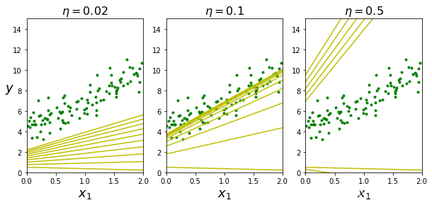

随机梯度下降

画图

theta_path_sgd = []
m = len(x_b)
np.random.seed(42)

n_epochs = 50

theta = np.random.randn(2,1) # 随机初始化

for epoch in range(n_epochs):
    for i in range(m):
        if epoch == 0 and i < 20:
            y_predict = x_new_b.dot(theta)
            style = "r-"
            plt.plot(x_new,y_predict,style)
        random_index = np.random.randint(m)
        xi = x_b[random_index:random_index+1]
        yi = y[random_index:random_index+1]
        gradients = 2 * xi.T.dot(xi.dot(theta) - yi)
        eta = 0.1
        theta = theta -eta * gradients
        theta_path_sgd.append(theta)
        
        
plt.plot(x,y,"g.")        
plt.xlabel("$x_1$",fontsize=18)
plt.ylabel("$y$",rotation=0,fontsize=18)
plt.axis([0,2,0,15])
save_fig("sgd_plot")  
plt.show()

结果：

Saving figure sgd_plot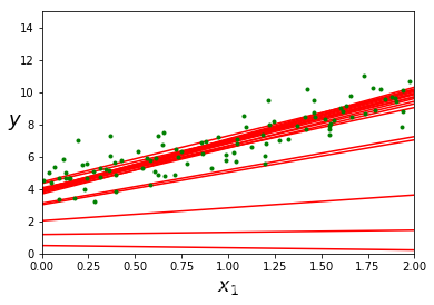

theta

结果：

array([[3.7625155],
[2.5892927]])

from sklearn.linear_model import SGDRegressor
sgd_reg = SGDRegressor(max_iter = 50,tol=np.infty,penalty=None,eta0=0.1,random_state=42)
sgd_reg.fit(x,y.ravel())

结果：

SGDRegressor(alpha=0.0001, average=False, early_stopping=False, epsilon=0.1,
eta0=0.1, fit_intercept=True, l1_ratio=0.15,
learning_rate=‘invscaling’, loss=‘squared_loss’, max_iter=50,
n_iter_no_change=5, penalty=None, power_t=0.25, random_state=42,
shuffle=True, tol=inf, validation_fraction=0.1, verbose=0,
warm_start=False)

sgd_reg.intercept_,sgd_reg.coef_

结果：

(array([4.25857953]), array([2.95762926]))

y

结果：

array([[ 6.33428778],
[ 9.40527849],
[ 8.48372443],
[ 5.60438199],
[ 4.71643995],
[ 5.29307969],
[ 5.82639572],
[ 8.67878666],
[ 6.79819647],
[ 7.74667842],
[ 5.03890908],
[10.14821022],
[ 8.46489564],
[ 5.7873021 ],
[ 5.18802735],
[ 6.06907205],
[ 5.12340036],
[ 6.82087644],
[ 6.19956196],
[ 4.28385989],
[ 7.96723765],
[ 5.09801844],
[ 5.75798135],
[ 5.96358393],
[ 5.32104916],
[ 8.29041045],
[ 4.85532818],
[ 6.28312936],
[ 7.3932017 ],
[ 4.68275333],
[ 9.53145501],
[ 5.19772255],
[ 4.64785995],
[ 9.61886731],
[ 7.87502098],
[ 8.82387021],
[ 5.88791282],
[ 7.0492748 ],
[ 7.91303719],
[ 6.9424623 ],
[ 4.69751764],
[ 5.80238342],
[ 5.34915394],
[10.20785545],
[ 6.34371184],
[ 7.06574625],
[ 7.27306077],
[ 5.71855706],
[ 7.86711877],
[ 7.29958236],
[ 8.82697144],
[ 8.08449921],
[ 9.73664501],
[ 8.86548845],
[ 6.03673644],
[ 9.59980838],
[ 3.4686513 ],
[ 5.64948961],
[ 3.3519395 ],
[ 7.50191639],
[ 5.54881045],
[ 5.30603267],
[ 9.78594227],
[ 4.90965564],
[ 5.91306699],
[ 8.56331925],
[ 3.23806212],
[ 8.99781574],
[ 4.70718666],
[10.70314449],
[ 7.3965179 ],
[ 3.87183748],
[ 4.55507427],
[ 9.18975324],
[ 8.49163691],
[ 8.72049122],
[ 7.94759736],
[ 4.67652161],
[ 6.44386684],
[ 3.98086294],
[11.04439507],
[ 8.21362168],
[ 4.79408465],
[ 5.03790371],
[ 4.89121226],
[ 6.73818454],
[ 9.53623265],
[ 7.00466251],
[10.28665258],
[ 7.24607048],
[ 5.53962564],
[10.17626171],
[ 8.31932218],
[ 6.61392702],
[ 7.73628865],
[ 6.14696329],
[ 7.05929527],
[ 6.90639808],
[ 4.42920556],
[ 5.47453181]])

y.ravel()

结果：

array([ 6.33428778, 9.40527849, 8.48372443, 5.60438199, 4.71643995,
5.29307969, 5.82639572, 8.67878666, 6.79819647, 7.74667842,
5.03890908, 10.14821022, 8.46489564, 5.7873021 , 5.18802735,
6.06907205, 5.12340036, 6.82087644, 6.19956196, 4.28385989,
7.96723765, 5.09801844, 5.75798135, 5.96358393, 5.32104916,
8.29041045, 4.85532818, 6.28312936, 7.3932017 , 4.68275333,
9.53145501, 5.19772255, 4.64785995, 9.61886731, 7.87502098,
8.82387021, 5.88791282, 7.0492748 , 7.91303719, 6.9424623 ,
4.69751764, 5.80238342, 5.34915394, 10.20785545, 6.34371184,
7.06574625, 7.27306077, 5.71855706, 7.86711877, 7.29958236,
8.82697144, 8.08449921, 9.73664501, 8.86548845, 6.03673644,
9.59980838, 3.4686513 , 5.64948961, 3.3519395 , 7.50191639,
5.54881045, 5.30603267, 9.78594227, 4.90965564, 5.91306699,
8.56331925, 3.23806212, 8.99781574, 4.70718666, 10.70314449,
7.3965179 , 3.87183748, 4.55507427, 9.18975324, 8.49163691,
8.72049122, 7.94759736, 4.67652161, 6.44386684, 3.98086294,
11.04439507, 8.21362168, 4.79408465, 5.03790371, 4.89121226,
6.73818454, 9.53623265, 7.00466251, 10.28665258, 7.24607048,
5.53962564, 10.17626171, 8.31932218, 6.61392702, 7.73628865,
6.14696329, 7.05929527, 6.90639808, 4.42920556, 5.47453181])

小批量梯度下降

theta_path_mgd = []

n_iterations = 50
minibatch_size = 20

np.random.seed(42)
theta = np.random.randn(2,1)


for epoch in range(n_iterations):
    shuffled_indices = np.random.permutation(m)
    x_b_shuffled = x_b[shuffled_indices]
    y_shuffled = y[shuffled_indices]
    for i in range(0,m,minibatch_size):
        xi = x_b_shuffled[i:i+minibatch_size]
        yi = y_shuffled[i:i+minibatch_size]
        gradients = 2/minibatch_size * xi.T.dot(xi.dot(theta) - yi)
        eta = 0.1
        theta = theta - eta * gradients
        theta_path_mgd.append(theta)
    

theta

结果：

array([[4.22023943],
[2.7704472 ]])

theta_path_bgd = np.array(theta_path_bgd)
theta_path_sgd = np.array(theta_path_sgd)
theta_path_mgd = np.array(theta_path_mgd)

plt.figure(figsize=(7,4))
plt.plot(theta_path_sgd[:, 0],theta_path_sgd[:, 1],"r-s",linewidth=1,label="Stochastic")
plt.plot(theta_path_mgd[:, 0],theta_path_mgd[:, 1],"g-+",linewidth=2,label="Mini-batch")
plt.plot(theta_path_bgd[:, 0],theta_path_bgd[:, 1],"b-o",linewidth=3,label="batch")
plt.legend(loc="upper left",fontsize = 16)
plt.xlabel(r"$\theta_0$",fontsize=20)
plt.ylabel(r"$\theta_1$",fontsize=20,rotation=0)
plt.axis([2.5,4.5,2.3,3.9])
save_fig("gradient_descent_paths_plot")  
plt.show()

结果：

Saving figure gradient_descent_paths_plot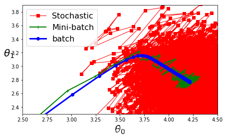

单独画出每个图

plt.plot(theta_path_sgd[:, 0],theta_path_sgd[:, 1],"r-s",linewidth=1,label="Stochastic")
plt.legend(loc="upper left",fontsize = 16)
plt.xlabel(r"$\theta_0$",fontsize=20)
plt.ylabel(r"$\theta_1$",fontsize=20,rotation=0)
plt.axis([2.5,4.5,2.3,3.9])
save_fig("gradient_descent_paths_plot")  
plt.show()

结果：

Saving figure gradient_descent_paths_plot

plt.plot(theta_path_mgd[:, 0],theta_path_mgd[:, 1],"g-+",linewidth=2,label="Mini-batch")
plt.legend(loc="upper left",fontsize = 16)
plt.xlabel(r"$\theta_0$",fontsize=20)
plt.ylabel(r"$\theta_1$",fontsize=20,rotation=0)
plt.axis([2.5,4.5,2.3,3.9])
save_fig("gradient_descent_paths_plot")  
plt.show()

结果：

Saving figure gradient_descent_paths_plot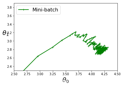

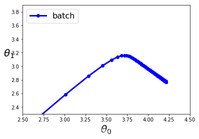
plt.plot(theta_path_bgd[:, 0],theta_path_bgd[:, 1],"b-o",linewidth=3,label="batch")
plt.legend(loc="upper left",fontsize = 16)
plt.xlabel(r"$\theta_0$",fontsize=20)
plt.ylabel(r"$\theta_1$",fontsize=20,rotation=0)
plt.axis([2.5,4.5,2.3,3.9])
save_fig("gradient_descent_paths_plot")  
plt.show()

结果：

Saving figure gradient_descent_paths_plot